The time step in all-atom simulations is usually of the order of the femtosecond (10-15 s). This means that a simulation running for 109 steps (which is already rather long) would make it possible to explore the dynamics of a system for timescales of the order of microseconds. With dedicated state-of-the-art hardware and very long simulations, small systems can be simulated for milliseconds, but going beyond that is prohibitive. What do we do if we want to explore phenomena with characteristic times that are significantly longer than these values? In this part[1] I will introduce you to some of the (countless) techniques that have been developed to answer this question.
The idea behind coarse-graining is to simplify complex systems by reducing the level of detail while retaining the physical and chemical properties of interest. There are both practical and conceptual advantages of CG models.
From the practical standpoint, by grouping atoms or molecules into larger units, coarse-graining enables the study of systems that would otherwise be computationally intractable at full atomistic resolution. The speed-up of CG models is due to several contributions:
The reduction of the number of degrees of freedom (e.g. atoms become CG sites, with ).
The smoothing of the potential energy function, which stems from the space averaging that is inherent to CG procedures and makes it possible to use (often much) larger time steps.
The forms of the interactions used in CG models, which are often simpler (e.g. no long-range interactions).
Implicit-solvent GC models have much less friction, leading to faster diffusion, and therefore a much more efficient sampling.
On a more conceptual level, reducing the number of degrees of freedom of a system can teach us something about the system itself. Indeed, CG models containing minimal sets of ingredients can be used to understand what are the ingredients underlying the phenomena of interest (Noid (2023)), which in many-body systems are often emergent properties, as famously discussed in the “More is different” paper by P. W. Anderson (Anderson (1972)).
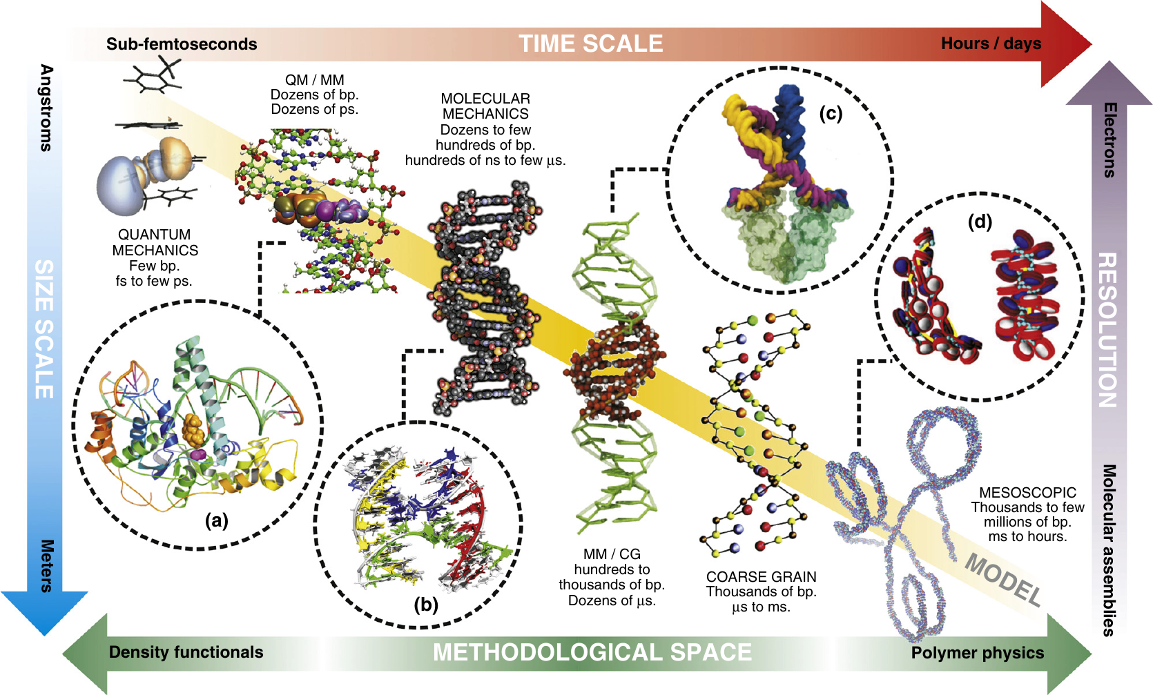
Figure 1:Models (here of DNA) with different levels of detail can be used to explore phenomena at different time and length scales. Taken from Dans et al. (2016).
As an example, Figure 1 shows some DNA models at different resolution, and the time and length scales that they can access in computer simulations.
A variety of approaches exist for creating coarse-grained models, which are often broadly categorised as either “top-down” or “bottom-up”. While the distinction between them is intuitive, many modern models blur these lines by integrating aspects of both philosophies.
A “bottom-up” CG model builds on a detailed, fine-grained (FG) model, which are often classical atomistic models rather than first principles. These models rely on statistical mechanics to reproduce thermodynamic and structural properties of the fine-grained system, using the many-body potential of mean force (see below for a more thorough discussion). While exact applications of this framework are, to date, impractical, all bottom-up models are nevertheless identified by the fact that they are derived from more detailed models.
Conversely, “top-down” models are based on experimental observations of phenomena at scales accessible to the CG model. These models are either generic, focusing on universal principles (e.g. scaling behaviour of polymers), or chemically specific, addressing particular systems. While they provide insights into emergent phenomena and large-scale behaviors, making it possible to trace their origin back to basic physical principles, they are not directly tied to more detailed models. As such, validating their assumptions or systematically improving them can be challenging. Unlike bottom-up models, which are constrained by detailed information, top-down models are often under-constrained by experimental data.
In the next sections I will introduce these two classes of models. I will use lowercase letters to refer to FG quantities (e.g. for the position of atom ), and uppercase letters to refer to CG quantities (e.g. for the position of CG bead ). The number of FG atoms and CG beads is and , respectively.
1Bottom-up models
Bottom-up coarse-grained (CG) models are constructed by systematically deriving interaction potentials from more detailed models, such as atomistic simulations, using principles of statistical mechanics. In these approaches, there is a systematic reduction of the degrees of freedom of the FG description that can be formally described by a (usually linear) mapping operator
An example would be describing each group of atoms with their centre of mass, in which case . Note that it is also possible to define mappings where some FG degrees of freedom are not used to define any CG variable (i.e. there are some atoms whose position is never used to compute any of the ). A classic example is provided by implicit-solvent models, where the CG variables are defined by the solute’s degrees of freedom only, and their interaction contains the effect of the solvent in an effective way. With Eq. (1), it is possible to map each FG configuration into a CG one, so that the overall FG equilibrium distribution turns into a “mapped distribution” given by
where the integration over the microscopic degrees of freedom is made explicit.
Once the mapping has been chosen (traditionally by intuition, but there are modern machine-learning approaches that try to automatise or assist this choice), the formal interaction between the new (CG) degrees of freedom is the many-body potential of mean force (PMF), also known as effective interaction, which can be formally written as
where is a constant. In principle, if the exact form of the CG potential is known at a given state point, then simulations using will reproduce the mapped distribution, Eq. (2), at that state point. Unfortunately, most of the times evaluating Eq. (3) analytically is not possible. There is a rather famous exception that I will mention, since some of you may be already familiar with it.
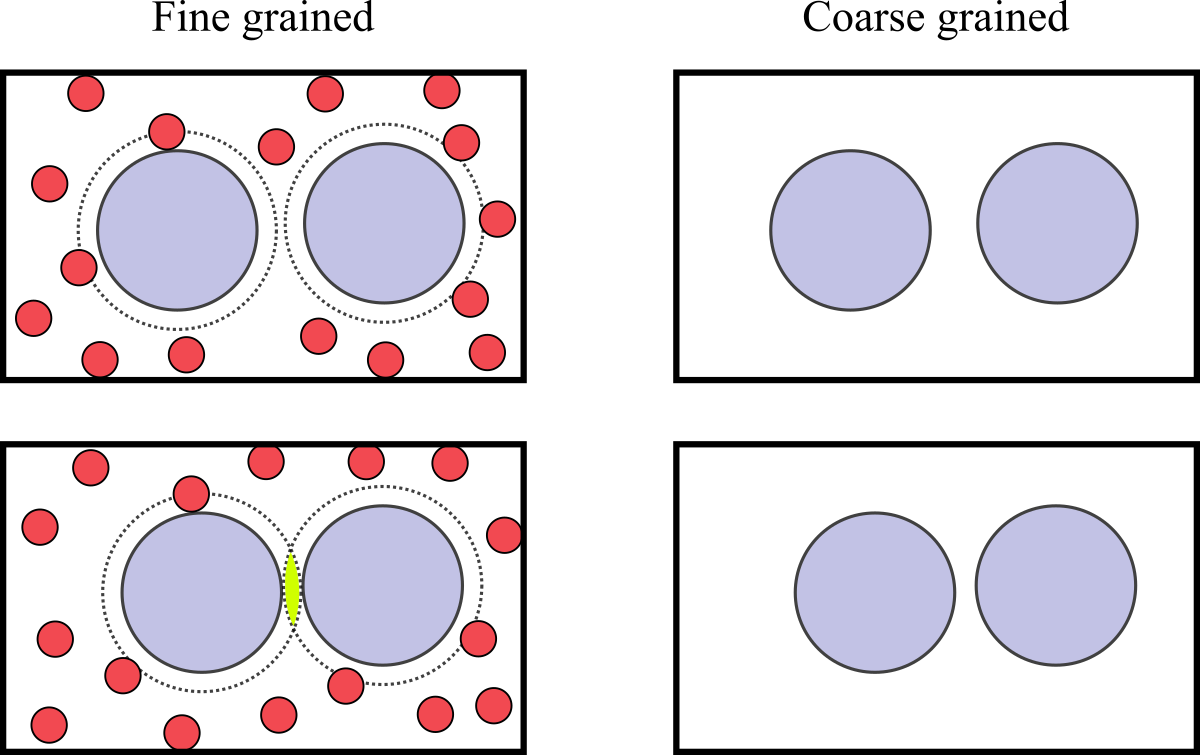
Figure 2:A mixture of large and small particles in a box. The left and right figures show the same configuration in the FG and CG descriptions, respectively. In the left panels, the dashed lines show the regions around large particles where small particles cannot enter. The bottom-left panel shows that, if the two large particles are close enough, their excluded regions overlap, giving raise to an effective interaction due to the larger volume accessible to the small particles.
The depletion interaction, which is ubiquitous in soft and biological matter (see e.g. Miyazaki et al. (2022)), arises when large and small particles are mixed together. As schematically shown in Figure 2, the effect is due to the larger volume that is accessible to the small particles if large particles get sufficiently close to each other. Using a simplified model, known as the Asakura-Oosawa (AO) model (see e.g. Oosawa (2021)), it is possible to directly apply Eq. (3) to derive the PMF.
In the AO model, large-large and small-large particles interact through excluded-volume repulsions, while small-small interactions are neglected. If we now define the CG variables as the positions of the large particles, the integration of Eq. (3) for the case of two large particles immersed in a “sea” of small particles having activity can be carried out exactly, yielding[2]
where is the diameter of the large particles, is the size ratio between small and large particles, and is the distance between the two large particles. Interestingly, it has been demonstrated (see e.g. Likos (2001) and references therein) that Eq. (4) is exact if , i.e. there are no higher-order terms in the PMF, even when the system contains more than two large particles[3].
In more general cases, the many-body effective interaction cannot be computed, so that it is common to resort to approximations, which most of the times amount to writing the integral appearing in Eq. (3) as a sum of contributions due to two-body, three-body, etc., interactions, and only retaining the first terms (often the two-body term only).
Many computational methods have been developed to estimate the PMF, or a “good-enough” approximation thereof. Here I will quickly present some of the ideas underlying these methods.
1.1Correlation Function Approaches
The correlation function approaches aim to parameterize coarse-grained effective potentials to reproduce specific structural properties, such as radial distribution functions, obtained from atomistic simulations. These methods often employ iterative techniques to refine the PMF, so that the CG model accurately represents the structural correlations of the atomistic system.
1.1.1Direct Boltzmann Inversion (DBI)
Direct Boltzmann Inversion is the simplest approach to derive CG potentials directly from atomistic distribution functions. For a pair interaction, the CG potential is given by:
where is the radial distribution function of the CG variables evaluated in the FG system. This potential corresponds to the pair potential of mean force, which effectively accounts for interactions mediated by the surrounding environment, and is exact only in the dilute limit, where many-body interactions are unlikely. Therefore, this method does not work well in dense systems, or systems where interactions are strongly coupled.
1.1.2Iterative Boltzmann Inversion (IBI)
To address the limitations of DBI, Iterative Boltzmann Inversion refines the potential iteratively. The goal is to adjust the CG potential until the radial distribution function of the CG model matches the atomistic one, so that the final pair PMF takes implicitly into account at least some of the many-body correlations that are present in the system. The iterative update for the potential is:
where is the RDF obtained by simulating the CG model interacting through , and is the target RDF.

Figure 3:Optimization of the intermolecular RDF for a melt of polyisoprene 9-mers by using IBI. The RDF of iteration 1 corresponds to the initial potential guess, the direct Boltzmann inversion of the intermolecular target RDF. The quality of the trial RDFs improves very fast. After the third iteration (shown), the trial RDFs match the target within line thickness (not shown any more). Taken from Reith et al. (2003).
This process continues until the two radial distribution functions converge within some accuracy. Figure 3 shows an example.
To conclude this part, I will mention that there exist other, often more refined, methods based on correlation function approaches, such as the Inverse Monte Carlo (IMC) approach, for which I refer you to Noid (2013) and references therein.
1.2Variational approaches
Variational approaches focus on systematically deriving a CG interaction potential by minimising a specific functional. In general, the approaches introduced here are very flexible, since the functionals to be minimised are independent of the specific form used to model the potential, and therefore there is great freedom in choosing how to optimise the PMF.
1.2.1Force-Matching
One of the most common variational approaches is force-matching, where the CG potential is parameterized to reproduce the forces observed in atomistic simulations. To determine the CG potential, the force-matching approach minimizes the sum of the squared differences between the FG force acting on each CG bead [4] and the force as computed by deriving the CG energy with respect to the position of bead , :
where is the PMF we wish to optimise, is the target PMF, the average is performed over the FG canonical ensemble, and .
Traditionally, Eq. (7) has been solved by expanding the CG potential in a chosen basis set, :
where are the coefficients to be determined, so that the minimization of with respect to the coefficients yields a linear system of equations, allowing the determination of the CG potential.
However, recently, machine-learning approaches have been employed to directly obtain the many-body PMF. The idea, introduced in Wang et al. (2019) is to use neural networks (NNs) to represent , since NNs can approximate any smooth function.
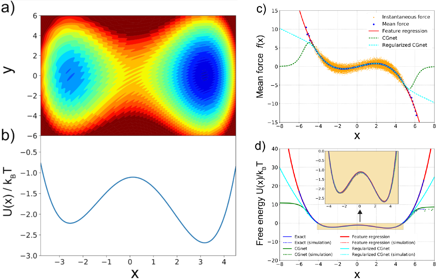
Figure 4:Machine-learned coarse-graining of dynamics in a rugged 2D potential. (a) Two-dimensional potential used as a toy system. (b) Exact free energy along . (c) Instantaneous forces and the learned mean forces compared to the exact forces. Here “feature regression” is a least-square fitting function, and regularized and unregularized CGnet models refer to NN models that treat the portions that are outside of the training data in different ways. The unit of force is , with the unit of length set to 1. (d) Free energy (PMF) along predicted using feature regression, and CGnet models compared to the exact free energy. Free energies are also computed from histogramming simulation data directly, using the underlying 2D trajectory, or simulations run with the feature regression and CGnet models (dashed lines). Taken from Wang et al. (2019).
Figure 4 shows a simple example, where the algorithm dubbed CGnet was able to learn the 1D representation of a “rugged” 2D interaction potential. The same technique has been applied to more realistic cases, such as proteins (Majewski et al. (2023), see Figure 5), or water (Guidarelli Mattioli et al. (2023)).
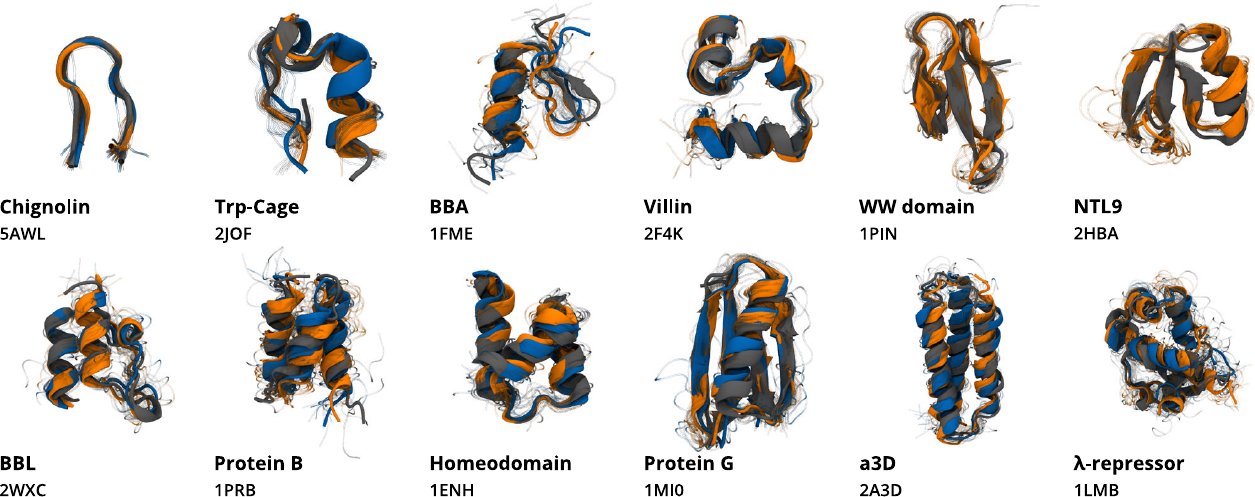
Figure 5:Structures obtained from CG simulations of the protein-specific model (orange) and the multi-protein model (blue), compared to their respective experimental structures (gray). Here the CG description retains only the position of the atoms. Taken from Majewski et al. (2023).
1.2.2Relative Entropy Minimization
An alternative variational approach minimizes the relative entropy, , between the atomistic and CG probability distributions, which is given by the so-called Kullback-Leibler (KL) divergence (introduced in Kullback & Leibler (1951)):
where and are the FG and (trial) CG distributions, respectively. vanishes only if (up to a constant). Interestingly, this approach has been shown to be equivalent to many of the methods that make use of correlation functions (such as IBI and IMC), in some sense providing a unified framework, as well as a theoretical justification, for these techniques (see Noid (2013) and references therein).
From an information theory point of view, the KL divergence can also be applied to estimate the loss of information associated to the coarse-graining procedure in itself. Indeed, by using the equilibrium distributions and in Eq. (9), it is possible to obtain a quantity that is function of the mapping operator only, . As suggested in Giulini et al. (2020), this quantity is a measure of the information content retained by the CG description. By minimising it, it is possible to find the optimal mapping that, given the chosen resolution, retains the maximum amount of information on the statistical properties of the FG system, or, in other words, the FG degrees of freedom (or the combinations thereof) that are more important in the determination of the behaviour of the original system.
2Top-down models
Top-down coarse-grained (CG) models derive their interactions from experimental observables or generic physical principles rather than atomistic-level details. Unlike bottom-up approaches, which aim to approximate the many-body potential of mean force (PMF) from a more detailed model, top-down models focus on reproducing emergent properties or large-scale behavior observed in experiments. These models are particularly useful for systems where fine-grained details are not critical, or when computational efficiency is a priority. An example we have seen is the HP model, where the idea was to develop a very fast model that retained the minimal set of ingredients required to reproduce some properties of the target system (i.e. the segregation of hydrophobic residues in the protein core, the formation of “ordered” secondary structure, etc.).
The philosophy behind top-down CG modeling can be categorized into two main types: generic and chemically specific. Generic models aim to capture universal physical principles without explicitly addressing the chemical identity of the system. They often use low-resolution representations and simplified potentials to explore broad phenomena, such as the role of hydrophobic interactions in protein folding or the impact of chain stiffness in DNA condensation. In contrast, chemically specific models target the properties of a specific system, such as a lipid bilayer or a particular protein, and are parameterized using experimental data. These models aim to reproduce observed structural or thermodynamic features, such as density, bilayer rigidity, or melting temperatures, by carefully tuning interaction potentials.
The derivation of top-down CG models begins with the selection of a coarse-grained representation, where “sites” are defined to represent groups of atoms or molecules. The choice of resolution depends on the phenomenon of interest—for example, treating entire proteins as single particles versus focusing on the behavior of individual amino acids. Once the representation is established, the interactions between these sites are parameterized. In generic models, this process is guided by physical intuition, with potentials chosen to explore specific features of the system, such as peptide secondary structure preferences. For chemically specific models, the parameterization process incorporates experimental data. The Martini model, for instance, assigns interaction strengths based on the partitioning behavior of compounds between aqueous and hydrophobic phases.
Given the philosophy summarised above, the derivation of top-down CG models cannot be done in a systematic way, as it mostly relies on physical intuition. Therefore, I will provide one example of a successful top-down model. This is a very biased example, since I have been working with (and, in part, developing) this particular model for more than 10 years.
2.1oxDNA/oxRNA
The oxDNA model was originally developed to study the self-assembly, structure and mechanical properties of DNA nanostructures, and the action of DNA nanodevices. However, it has since been applied more broadly. To describe such systems, a model needs to capture the structural, mechanical and thermodynamic properties of single-stranded DNA, double-stranded DNA, and the transition between the two states. It must also be feasible to simulate large enough systems for long enough to sample the key phenomena. Mesoscopic models, in which multiple atoms are represented by a single interaction site, are the appropriate resolution for these goals.
Here I will outline the key features of the oxDNA model. First of all, note that there are effectively three versions of the oxDNA potential that are publicly available. The original model, oxDNA1.0 (Ouldridge et al. (2011)), lacks sequence-specific interaction strengths, electrostatic effects and major/minor grooving. oxDNA1.5 adds sequence-dependent interaction strengths to oxDNA1.0 (Šulc et al. (2012)), and oxDNA2.0 (Snodin et al. (2015)) also includes a more accurate structural model, alongside an explicit term in the potential for screened electrostatic interactions between negatively charged sites on the nucleic acid backbone. In addition to these three versions of the DNA model, an RNA parameterisation, oxRNA, has also been introduced (Šulc et al. (2014)).
It is worth noting that the three versions of oxDNA are very similar; most of the changes involve small adjustments of the geometry and strength of interactions. Structurally, the most significant change is the addition of a screened electrostatic interaction in oxDNA 2.0, which is typically small unless low salt concentrations are used. Moreover, subsequent versions of the model have been explicitly designed to preserve aspects of earlier versions that performed well. So oxDNA 1.5 and oxDNA 1.0 are very similar, except that oxDNA predicts sequence-dependent thermodynamic effects that are absent in oxDNA 1.0. oxDNA 2.0 is designed to preserve the thermodynamic and mechanical properties of oxDNA 1.5 at high salt as far as possible, but improves the structural description of duplexes (and structures built from duplexes) and allows for accurate thermodynamics at lower salt concentrations. There is also a model for RNA, introduced in Šulc et al. (2014) and dubbed oxRNA, which is based on the same principles of, although it has slightly worse thermodynamics-wise performance than, oxDNA. This is mostly due to the fact that non-canonical base pairing mechanisms, which are missing in oxDNA/oxRNA, are more important in RNA than DNA.
As a result, therefore, the discussion provided here for simulation of one version of the model largely applies to all. Moreover, it is worth noting that, even given the improved accuracy of oxDNA 2.0 in certain contexts, simulations of the 1.5 version of the model are still potentially valuable. oxDNA 2.0 comes into its own when it is essential to incorporate longer-range electrostatics at low salt concentrations, or when the detailed geometry of the helices are particularly important. A good example would be when simulating densely packed helices connected by crossover junctions in DNA origami. In other contexts, the reduced complexity of oxDNA 1.5 and hence its improved computational efficiency (along with slightly greater focus on basic thermodynamics and mechanics) may be beneficial. Since there is also a sequence-independent oxDNA 1.5 version, it usually makes little sense to use oxDNA 1.0.
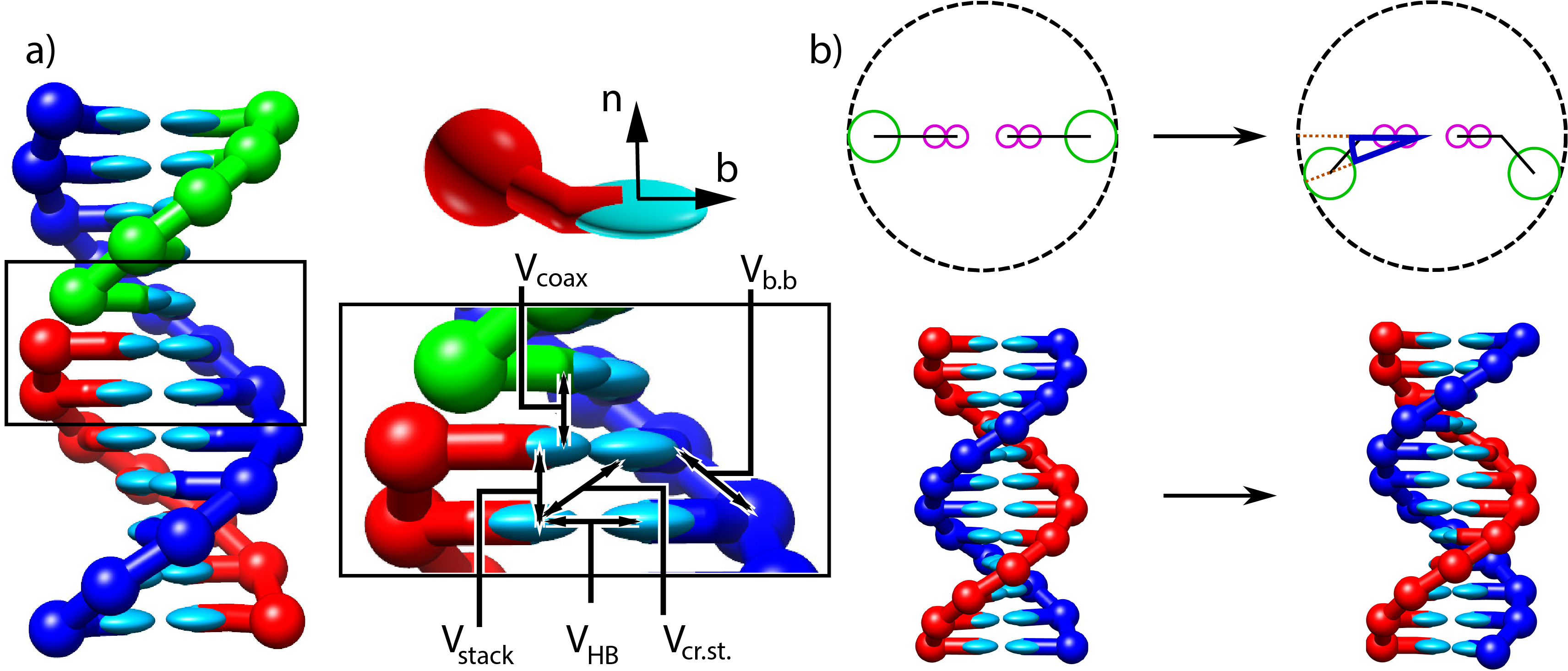
Figure 6:Structure and interactions of the oxDNA model. a) Three strands forming a nicked duplex as represented by oxDNA2.0, with the central section of the complex illustrating key interactions from Eq. (10) highlighted. Individual nucleotides have an orientation described by a vector normal to the plane of the base (labelled n), and a vector indicating the direction of the hydrogen bonding interface (labelled b). b) Comparison of structure in oxDNA1.0 and oxDNA1.5 vs oxDNA2.0. In the earlier version of the model, all interaction sites are co-linear; in oxDNA2.0, offsetting the backbone site allows for major and minor grooving. Taken from Sengar et al. (2021).
In all three parameterisations, oxDNA represents each nucleotide as a rigid body with several interaction sites, namely the backbone, base repulsion, stacking and hydrogen-bonding sites, as shown in Figure 6. In oxDNA1.0 and oxDNA1.5, these sites are co-linear; the more realisic geometry of oxDNA2.0 offsets the backbone to allow for major and minor grooving.
Interactions between nucleotides depend on the orientation of the nucleotides as a whole, rather than just the position of the interaction sites. In particular, there is a vector that is perpendicular to the notional plane of the base, and a vector that indicates the direction of the hydrogen bonding interface. These vectors are used to modulate the orientational dependence of the interactions, which allows the model to represent the coplanar base stacking, the linearity of hydrogen bonding and the edge-to-edge character of the Watson–Crick base pairing. Furthermore, this representation allows the encoding of more detailed structural features of DNA, for example, the right-handed character of the double helix and the anti-parallel nature of the strands in the helix.
The potential energy of the system is calculated as:
with an additional screened electrostatic repulsion term for oxDNA 2.0. In Eq. (10), the first sum is taken over all pairs of nucleotides that are nearest neighbors on the same strand and the second sum comprises all remaining pairs. The terms represent backbone connectivity (), excluded volume ( and ), hydrogen bonding between complementary bases (), stacking between adjacent bases on a strand (), cross-stacking () across the duplex axis and coaxial stacking () across a nicked backbone. The excluded volume and backbone interactions are a function of the distance between repulsion sites. The backbone potential is a spring potential mimicking the covalent bonds along the strand. All other interactions depend on the relative orientations of the nucleotides and the distance between the hydrogen-bonding and stacking interaction sites. The model was deliberately constructed with all interactions pairwise (i.e., only involving two nucleotides, which are taken as rigid bodies).
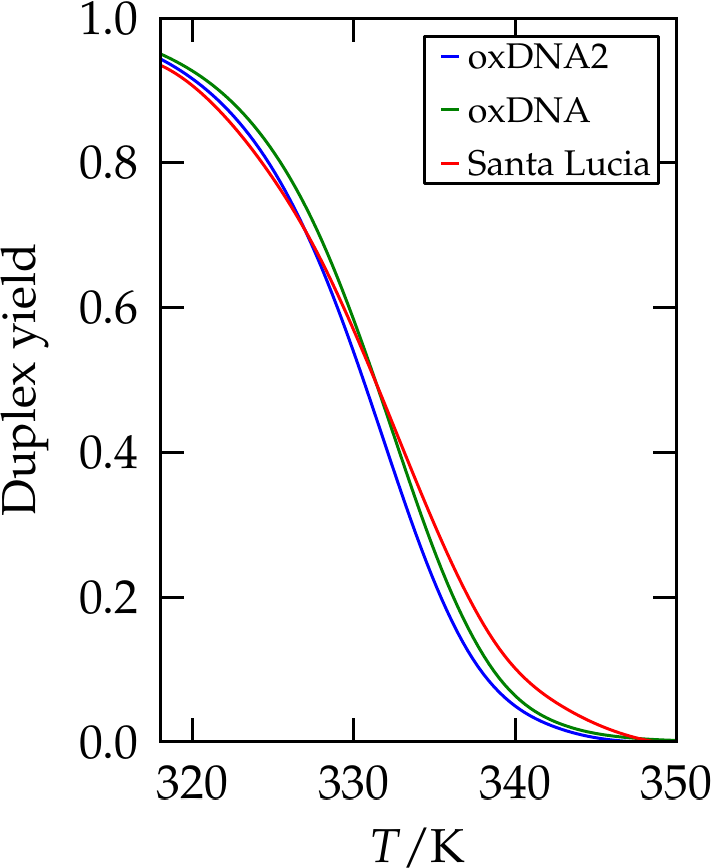
Figure 7:The yield of a 10-bp duplex as predicted by SantaLucia (red line), compared with results from oxDNA and oxDNA2. Adapted from Snodin et al. (2015).
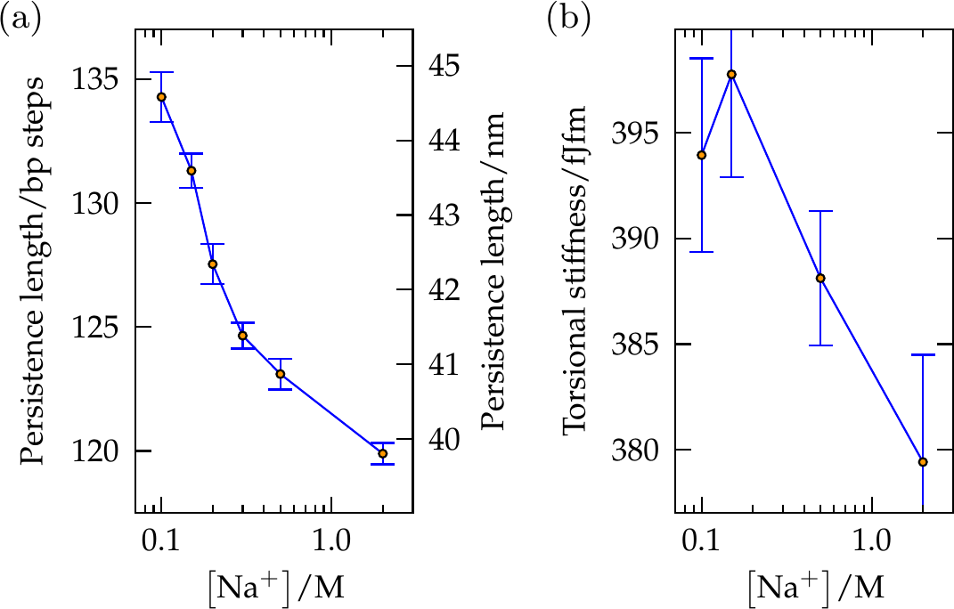
Figure 8:(a) The persistence length and (b) the torsional stiffness of duplex DNA in oxDNA2 as a function of salt concentration. These values are consistent with experiments. Taken from Snodin et al. (2015).
A crucial feature of the oxDNA model is that the double helical structure is driven by the interplay between the hydrogen-bonding, stacking and backbone connectivity bonds. The stacking interaction tends to encourage the nucleotides to form co-planar stacks; the fact that this stacking distance is shorter than the backbone bond length results in a tendency to form helical stacked structures. In the single-stranded state, these stacks can easily break, allowing the single strands to be flexible. The geometry of base pairing with a complementary strand locks the nucleotides into a much more stable double helical structure. Note that oxDNA and oxRNA have been parametrised to reproduce the thermodynamics of nearest-neighbour models, see Figure 7, as well as the experimental bending and torsional flexibility of the molecules, see Figure 8.
It is convenient to use reduced units to describe lengths, energies and times in the system. Here is a summary of the conversion of these “oxDNA units” to SI units:
One unit of length corresponds to 8.518 . This value was chosen to give a rise per bp of approximately 3.4 and equates roughly to the diameter of a nucleotide.
One unit of energy is equal to = 4.142 J (or equivalently, at = 300 K corresponds to 0.1).
The cutoff for treating two bases as “stacked” or “base-paired” is conventionally taken to be when the relevant interaction term is more negative than -0.1 in simulation units ( J).
The units of energy and length imply a simulation unit of force equal to N.
oxDNA and oxRNA can be simulated by using the standalone code, which contains documentation and many examples you can use to familiarise with it. Sample et al. (2023) (also available as a preprint here) is a very useful tutorial that answers the question “Where should I start if I want to use oxDNA”.
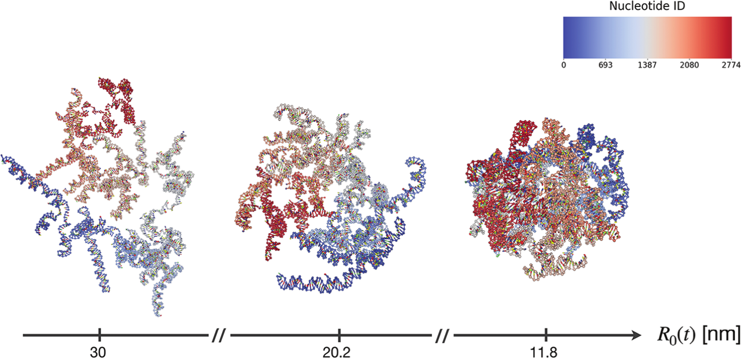
Figure 9:Snapshots of configurations of the RNA2 fragment of the CCMV virus, squeezed by a sphere of a radius given by 30, 20.2 and 11.8 nm (from left to right). The color scale is associated with the nucleotide index. Taken from Mattiotti et al. (2024).
As a recent example, oxRNA has been used to study the conformational ensemble of a viral RNA comprising almost 3000 nucleotides. Thanks to lengthy simulations, in Mattiotti et al. (2024) it was possible to test some theoretical predictions, as well as to see the effect of the confinement due to the viral capsid. Figure 9 shows some representative simulation snapshots.
In some sense, also the next part will be dedicated to answering this question, but from another point of view.
See Francesco Sciortino’s notes for details.
The value of has a geometric explanation: indeed, if , a small sphere can pass through the free space formed by three large spheres put in contact with each other in an equilateral configuration.
if the mapping is linear.
- Noid, W. G. (2013). Perspective: Coarse-grained models for biomolecular systems. The Journal of Chemical Physics, 139(9). 10.1063/1.4818908
- Noid, W. G. (2023). Perspective: Advances, Challenges, and Insight for Predictive Coarse-Grained Models. The Journal of Physical Chemistry B, 127(19), 4174–4207. 10.1021/acs.jpcb.2c08731
- Anderson, P. W. (1972). More Is Different: Broken symmetry and the nature of the hierarchical structure of science. Science, 177(4047), 393–396. 10.1126/science.177.4047.393
- Dans, P. D., Walther, J., Gómez, H., & Orozco, M. (2016). Multiscale simulation of DNA. Current Opinion in Structural Biology, 37, 29–45. 10.1016/j.sbi.2015.11.011
- Miyazaki, K., Schweizer, K. S., Thirumalai, D., Tuinier, R., & Zaccarelli, E. (2022). The Asakura–Oosawa theory: Entropic forces in physics, biology, and soft matter. The Journal of Chemical Physics, 156(8). 10.1063/5.0085965
- Oosawa, F. (2021). The history of the birth of the Asakura–Oosawa theory. The Journal of Chemical Physics, 155(8). 10.1063/5.0049350
- Likos, C. N. (2001). Effective interactions in soft condensed matter physics. Physics Reports, 348(4–5), 267–439. 10.1016/s0370-1573(00)00141-1
- Reith, D., Pütz, M., & Müller‐Plathe, F. (2003). Deriving effective mesoscale potentials from atomistic simulations. Journal of Computational Chemistry, 24(13), 1624–1636. 10.1002/jcc.10307
- Wang, J., Olsson, S., Wehmeyer, C., Pérez, A., Charron, N. E., de Fabritiis, G., Noé, F., & Clementi, C. (2019). Machine Learning of Coarse-Grained Molecular Dynamics Force Fields. ACS Central Science, 5(5), 755–767. 10.1021/acscentsci.8b00913
- Majewski, M., Pérez, A., Thölke, P., Doerr, S., Charron, N. E., Giorgino, T., Husic, B. E., Clementi, C., Noé, F., & De Fabritiis, G. (2023). Machine learning coarse-grained potentials of protein thermodynamics. Nature Communications, 14(1). 10.1038/s41467-023-41343-1
- Guidarelli Mattioli, F., Sciortino, F., & Russo, J. (2023). A neural network potential with self-trained atomic fingerprints: A test with the mW water potential. The Journal of Chemical Physics, 158(10). 10.1063/5.0139245
- Kullback, S., & Leibler, R. A. (1951). On Information and Sufficiency. The Annals of Mathematical Statistics, 22(1), 79–86. 10.1214/aoms/1177729694
- Giulini, M., Menichetti, R., Shell, M. S., & Potestio, R. (2020). An Information-Theory-Based Approach for Optimal Model Reduction of Biomolecules. Journal of Chemical Theory and Computation, 16(11), 6795–6813. 10.1021/acs.jctc.0c00676
- Marrink, S. J., & Tieleman, D. P. (2013). Perspective on the Martini model. Chemical Society Reviews, 42(16), 6801. 10.1039/c3cs60093a
- Sengar, A., Ouldridge, T. E., Henrich, O., Rovigatti, L., & Šulc, P. (2021). A Primer on the oxDNA Model of DNA: When to Use it, How to Simulate it and How to Interpret the Results. Frontiers in Molecular Biosciences, 8. 10.3389/fmolb.2021.693710