Using oxDNA from Python - Notes for the Computational Biophysics class

Here I will show you how to run an oxDNA simulation, visualising configurations with oxView and analysing the results.

Download oxDNA
Compile it:

cd oxDNA
mkdir build
cd build
cmake .. -DPython=On
make install -j6

If you want to run this notebook, download the oxDNA_input, hairpin.conf and hairpin.top files (and rename them so that they retain their original name).

# clean up all files from the previous run
!rm trajectory.dat
!rm energy.dat
!rm *.pyidx
!rm relax_energy.dat
!rm bonds*
p = None

rm: cannot remove 'trajectory.dat': No such file or directory
zsh:1: no matches found: *.pyidx
rm: cannot remove 'relax_energy.dat': No such file or directory
zsh:1: no matches found: bonds*

We can visualise the initial configuration using oxView.

# all functions required to read a configuration using the new RyeReader
from oxDNA_analysis_tools.UTILS.RyeReader import describe, get_confs, inbox
# the function used to visualize a configuration in oxView
from oxDNA_analysis_tools.UTILS.oxview import oxdna_conf

top = "./hairpin.top"
traj = "./hairpin.conf"
input_file = "./oxDNA_input"
# RyeReader uses indexing allows for random access in the trajectory
top_info, traj_info = describe(top, traj)

# This is the new way to read configurations, as it returns a list we need [0]
# to access a single conf
ref_conf = get_confs(top_info, traj_info, 0, 1)[0]
# inbox the configuration
ref_conf = inbox(ref_conf)

# show an iframe displaying the configuration
# inbox_settings = ["None", "None"] makes sure oxview does no post processing of the
# loaded configuration
oxdna_conf(top_info, ref_conf, inbox_settings=["None","None"])

WARNING: The old topology format is depreciated and future tools may not support it.  Please update to the new topology format for future simulations.

Our system is a short strand that can form a hairpin. We will run a short relaxation simulation. Note that the simulation is run on a separate thread, so during the run it is possible to run the analysis cells down the book. In principle, this also allows to run more than one replica at a time.

import oxpy
import multiprocessing
# define the number of simulation steps we run
STEPS = 2000000
INTERVAL = 10000
dt = 0.003

# helper function offloading the work to a new process
def spawn(f, args = ()):
    p = multiprocessing.Process(target=f, args= args )
    p.start()
    return p

# one simulation instance
# if you want to have multiple make sure the output files are different 
def relax_replica():
    with oxpy.Context():
        input = oxpy.InputFile()
        input.init_from_filename(input_file)
        # all input parameters provided to oxDNA need to be strings 
        input["steps"] = str(STEPS)
        input["print_conf_interval"] = str(INTERVAL)
        input["print_energy_every"] = str(INTERVAL)
        input["dt"] = str(dt)
        # make sure our output is not overcrowded
        input["no_stdout_energy"] = "true"
        # these settings turn a regular simulation into a relaxation one  
        input["T"] = "10C"
        input["max_backbone_force"] = "5"
        input["max_backbone_force_far"] = "10"
        input["energy_file"] = "relax_energy.dat"
        # discard the relax data and log info
        input["trajectory"] = "/dev/null"
        input["log_file"] = "/dev/null"

        # init the manager with the given input file
        manager = oxpy.OxpyManager(input)
        #run complete run's it till the number steps specified are reached 
        manager.run_complete()

# make sure we don't have anything running
try:
    p.terminate()
except:
    pass
# run a simulation and obtain a reference to the background process
p = spawn(relax_replica)

WARNING: Overwriting key `diff_coeff' (`2.5' to `2.5')
WARNING: Overwriting key `steps' (`1000000' to `2000000')
WARNING: Overwriting key `print_conf_interval' (`10000' to `10000')
WARNING: Overwriting key `print_energy_every' (`10000' to `10000')
WARNING: Overwriting key `dt' (`0.003' to `0.003')
WARNING: Overwriting key `T' (`60.85C' to `10C')
WARNING: Overwriting key `energy_file' (`energy.dat' to `relax_energy.dat')

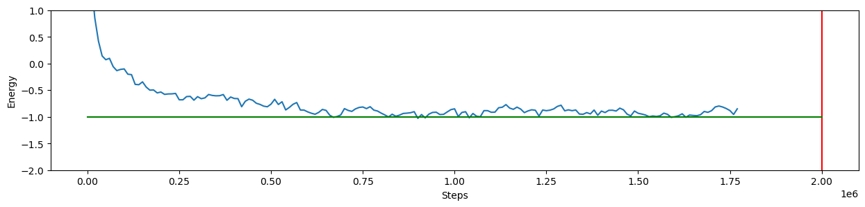
Since the simulation is run on a different thread, we can plot the energy while the simulation is running. W will be runnin a MD relaxation simulation, so the energy file format is:

[time (steps)] [Total Energy] [Potential Energy] [Kinetic Energy]

We add at the end a vertical line to indicate the length of the simulation, and since we are looking at an unformed hairpin, a “good” relaxed energy would be around -1, which is the green line.

The cell can be reloaded multiple times during the running simulation to see progress.

import pandas as pd
import matplotlib.pyplot as plt
df = pd.read_csv("relax_energy.dat", delimiter="\s+",names=['time', 'U','P','K'])

# make sure our figure is bigger
plt.figure(figsize=(15,3)) 
# plot the energy
plt.plot(df.time/dt,df.U)
# and the line indicating the complete run
plt.ylim([-2,1])
plt.plot([STEPS,STEPS],[df.U.max(),df.U.min()-2], color="r")
plt.ylabel("Energy")
plt.xlabel("Steps")
# and the relaxed state line
plt.plot([0, STEPS], [-1,-1], color="g")
print("Relaxation is running:", p.is_alive())

Relaxation is running: True

Now we can have a look at the last configuration

#load and inbox
ti, di = describe(top, "./last_conf.dat")
conf = inbox(get_confs(ti,di, 0,1)[0])
# display
oxdna_conf(ti, conf, inbox_settings=["None","None"])

WARNING: The old topology format is depreciated and future tools may not support it.  Please update to the new topology format for future simulations.

The melting temperature of this specific hairpin is 60.85 C, which means that at this temperature it is most probable that the hairpin will transition between a fully bonded state and fully melted.

STEPS = 60000000
INTERVAL = 50000
# define our boiler plate code to run the simulation
def replica():
    with oxpy.Context():
        input = oxpy.InputFile()
        input.init_from_filename(input_file)
        # all input parameters provided to oxDNA need to be strings 
        input["conf_file"] = "last_conf.dat"
        input["steps"] = str(STEPS)
        input["print_conf_interval"] = str(INTERVAL)
        input["print_energy_every"] = str(INTERVAL)
        input["dt"] = str(dt)
        # make sure our output is not overcrowded
        input["no_stdout_energy"] = "true"
        input["log_file"] = "log_production.dat"
        
        # init the manager with the given input file
        manager = oxpy.OxpyManager(input)
        #run complete run's it till the number steps specified are reached 
        manager.run_complete()

#make sure we don't have anything running
try:
    p.terminate()
except:
    pass
#note that for more than one replica running you will have to change the guard code 
spawn(replica)

WARNING:

<Process name='Process-5' pid=1548511 parent=1538542 started>

Overwriting key `diff_coeff' (`2.5' to `2.5')
WARNING: Overwriting key `conf_file' (`hairpin.conf' to `last_conf.dat')
WARNING: Overwriting key `steps' (`1000000' to `60000000')
WARNING: Overwriting key `print_conf_interval' (`10000' to `50000')
WARNING: Overwriting key `print_energy_every' (`10000' to `50000')
WARNING: Overwriting key `dt' (`0.003' to `0.003')
INFO: seeding the RNG with 1503251921
INFO: Initializing backend 
INFO: Simulation type: MD
INFO: The generator will try to take into account bonded interactions by choosing distances between bonded neighbours no larger than 2.000000
INFO: Converting temperature from Celsius (60.850000 C°) to simulation units (0.111333)
INFO: Running Debye-Huckel at salt concentration =  1
INFO: Using different widths for major and minor grooves
INFO: Temperature change detected (new temperature: 60.85 C, 334.00 K), re-initialising the DNA interaction
DEBUG: Debye-Huckel parameters: Q=0.054300, lambda_0=0.361646, lambda=0.381589, r_high=1.144767, cutoff=2.679947
DEBUG: Debye-Huckel parameters: debye_huckel_RC=1.717150e+00, debye_huckel_B=7.208180e-03
INFO: The Debye length at this temperature and salt concentration is 0.381589
INFO: pid: 1548511
DEBUG: Debye-Huckel parameters: Q=0.054300, lambda_0=0.361646, lambda=0.381589, r_high=1.144767, cutoff=2.679947
DEBUG: Debye-Huckel parameters: debye_huckel_RC=1.717150e+00, debye_huckel_B=7.208180e-03
INFO: The Debye length at this temperature and salt concentration is 0.381589
INFO: (Cells.cpp) N_cells_side: 4, 4, 4; rcut=3.07995, IS_MC: 0
INFO: N: 18, N molecules: 1
INFO: Using randomly distributed velocities
INFO: Initial kinetic energy: 5.571667
INFO: diffusion fixed.. -14.8859 -14.8859
INFO: diffusion fixed.. -12.6048 -12.6048
INFO: diffusion fixed.. -10.8525 -10.8525
INFO: diffusion fixed.. -11.3755 -11.3755
INFO: diffusion fixed.. -12.8351 -12.8351
INFO: diffusion fixed.. -11.3582 -11.3582
INFO: diffusion fixed.. -13.8222 -13.8222

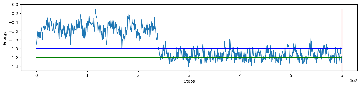
Here we can monitor the energy as before, but I add two lines to the output, to distinguish the two possibilities:

Energy $\approx -1$ corresponds to the open structure (blue line)
Energy $\approx -1.2$ is a fully bonded hairpin (green line)

The visualization will appear only if the simulation has completed, and it is the last configuration with computed bond energy per nucleotide

import pandas as pd
import matplotlib.pyplot as plt
df = pd.read_csv("energy.dat", delimiter="\s+", names=['time', 'U','P','K'])

# make sure our figure is bigger
plt.figure(figsize=(15,3)) 
# plot the energy
plt.plot(df.time/dt, df.U)
# and the line indicating the complete run
plt.ylim([-1.5,0])
plt.plot([STEPS,STEPS], [df.U.max(), df.U.min()-2], color="r")
plt.ylabel("Energy")
plt.xlabel("Steps")
# and the relaxed state line
plt.plot([0, STEPS], [-1, -1], color="b")
plt.plot([0, STEPS], [-1.2, -1.2], color="g")
print("Simulation is running:", p.is_alive())
plt.show()


#load last conf
ti, di = describe(top, "./last_conf.dat")
conf = get_confs(ti,di, 0,1)[0]
print("Last configuration is:")

#produce the hydrogen bond overlay
!oat output_bonds -v bonds -p 2 oxDNA_input last_conf.dat

from json import loads
with open("bonds_total.json") as file:
    overlay = loads(file.read())

# display
oxdna_conf(ti, conf, overlay=overlay)

Simulation is running: False

Last configuration is:
INFO: oxDNA_analysis_tools version: 2.5.0
INFO: running config.py installed at: /home/lorenzo/.local/lib/python3.11/site-packages/oxDNA_analysis_tools/config.py
INFO: Python version: 3.11.9
INFO: Package Numpy found. Version: 1.26.4
INFO: Package oxpy found. Version: 3.6.2.dev78+ga20df96a.d20241108
INFO: No dependency issues found.
INFO: no units specified, assuming oxDNA su
WARNING: Overwriting key `diff_coeff' (`2.5' to `2.5')
WARNING: Overwriting key `trajectory_file' (`trajectory.dat' to `/home/lorenzo/Dropbox/ROMA/INSEGNAMENTO/COMPUTATIONAL_BIOPHYSICS/LEZIONI/comp_bio_notes/notebooks/last_conf.dat')
INFO: The generator will try to take into account bonded interactions by choosing distances between bonded neighbours no larger than 2.000000
INFO: Converting temperature from Celsius (60.850000 C°) to simulation units (0.111333)
INFO: Running Debye-Huckel at salt concentration =  1
INFO: Using different widths for major and minor grooves
DEBUG: Debye-Huckel parameters: Q=0.054300, lambda_0=0.361646, lambda=0.381589, r_high=1.144767, cutoff=2.679947
DEBUG: Debye-Huckel parameters: debye_huckel_RC=1.717150e+00, debye_huckel_B=7.208180e-03
INFO: The Debye length at this temperature and salt concentration is 0.381589
INFO: (Cells.cpp) N_cells_side: 4, 4, 4; rcut=2.67995, IS_MC: 0
INFO: N: 18, N molecules: 1

Please cite at least the following publication for any work that uses the oxDNA simulation package
  * E. Poppleton et al., J. Open Source Softw. 8, 4693 (2023), DOI: 10.21105/joss.04693
INFO: Aggregated I/O statistics (set debug=1 for file-wise information)
	  0.000  B written to files
	  0.000  B written to stdout/stderr
INFO: Processing in blocks of 20 configurations
INFO: You can modify this number by running oat config -n <number>, which will be persistent between analyses.
INFO: Starting up 2 processes for 1 chunks
INFO: All spawned, waiting for results
WARNING: Overwriting key `diff_coeff' (`2.5' to `2.5')
WARNING: Overwriting key `trajectory_file' (`trajectory.dat' to `/home/lorenzo/Dropbox/ROMA/INSEGNAMENTO/COMPUTATIONAL_BIOPHYSICS/LEZIONI/comp_bio_notes/notebooks/last_conf.dat')

WARNING: The old topology format is depreciated and future tools may not support it.  Please update to the new topology format for future simulations.

INFO: The generator will try to take into account bonded interactions by choosing distances between bonded neighbours no larger than 2.000000
INFO: Running Debye-Huckel at salt concentration =  1
INFO: Using different widths for major and minor grooves
DEBUG: Debye-Huckel parameters: Q=0.054300, lambda_0=0.361646, lambda=0.381589, r_high=1.144767, cutoff=2.679947
DEBUG: Debye-Huckel parameters: debye_huckel_RC=1.717150e+00, debye_huckel_B=7.208180e-03
INFO: The Debye length at this temperature and salt concentration is 0.381589
INFO: (Cells.cpp) N_cells_side: 4, 4, 4; rcut=2.67995, IS_MC: 0
INFO: N: 18, N molecules: 1

Please cite at least the following publication for any work that uses the oxDNA simulation package
  * E. Poppleton et al., J. Open Source Softw. 8, 4693 (2023), DOI: 10.21105/joss.04693
INFO: Aggregated I/O statistics (set debug=1 for file-wise information)
	  0.000  B written to files
	  0.000  B written to stdout/stderr
finished 1/1
INFO: Wrote oxView overlay to: bonds_FENE.json
INFO: Wrote oxView overlay to: bonds_BEXC.json
INFO: Wrote oxView overlay to: bonds_STCK.json
INFO: Wrote oxView overlay to: bonds_NEXC.json
INFO: Wrote oxView overlay to: bonds_HB.json
INFO: Wrote oxView overlay to: bonds_CRSTCK.json
INFO: Wrote oxView overlay to: bonds_CXSTCK.json
INFO: Wrote oxView overlay to: bonds_DH.json
INFO: Wrote oxView overlay to: bonds_total.json