1Proteins
Let’s consider a 100-residue peptide chain with a unique folded state. If each amino acid had only two available conformations, the number of configurations available to the chain would be . If the time required to switch between any two configurations was 10-12 s (a picosecond), and we assume that no configuration is visited twice, it would take approximately 1018 seconds to explore all the “phase space” (and therefore, on average, to fold): this is close to the age of the universe! In reality, proteins fold on time scales ranging from microseconds to hours. This is the gist of the famous “Levinthal’s paradox”, which implies that the search for the folded structure does not happen randomly, but it is guided by the energy surface of residue-residue interactions.
Proteins can be denatured by changing the solution conditions. Very high or low temperature and pH, or high concentration of a denaturant (like urea or guanine dihydrochloride) can “unfold” a protein, which loses its solid-like, native structure, as well as its ability to perform its biological function. Investigations of the unfolding of small globular proteins showed that, as the denaturing agent (e.g. temperature or denaturant concentration) increases, many of the properties of the protein go through an “S-shaped” change, which is characteristic of cooperative transitions.
Furthermore, calorimetric studies show that the denaturation transition is an “all-or-none” transition, i.e. that the “melting unit” of the transition is the protein as a whole, and not some subparts. This of course applies to single-domain small proteins, or to the single domains of larger proteins. Here “all-or-none” means that the protein exist only in one of two states (native or denaturated), with all the other “intermediate” states being essentially unpopulated at equilibrium. Therefore, this transition is the microscopic equivalent of a first-order phase transition (e.g. boiling or melting) occurring in a macroscopic system. Of course, since proteins are finite systems and therefore very far from the thermodynamic limit, this is not a true phase transition, as the energy jump is continuous, and the transition width is finite.
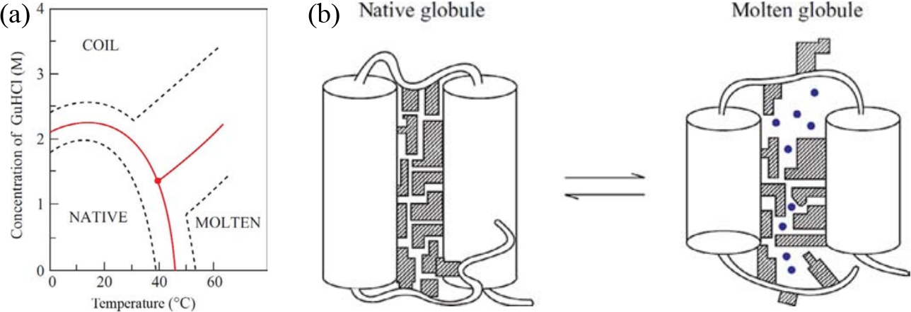
Figure 1:(a) Phase diagram of the conformational states of lysozyme at pH 1.7 as a function of denaturant (guanine dihydrochloride) concentration and temperature. The red lines correspond to the mid transition, the dashed lines outline the transition zones. (b) Schematic model of the native and molten globule protein states. Here the protein consists of only two helices connected by a loop, and the side chains are shown as shaded regions. Adapted from Finkelstein & Ptitsyn (2002).
But how does the denatured state look like? As discovered by using a plethora of experimental methods, which often seemed contradicting each other, the answer depends on the denaturing conditions. Figure 1(a) shows the phase diagram of lysozyme (a globular small protein) for different temperatures and concentrations of a denaturing agent. Increasing the latter leads to a transition to a disordered coil state where essentially no secondary structure is present. By contrast, the effect of temperature is qualitatively different, as the protein partially melts in a state (the molten globule, MG) that retains most of its secondary structure, but it is not solid like and it cannot perform any biological function. A schematic of the difference between the native and molten globule states is shown in Figure 1(b).
The cooperative transition that leads to the molten globule is due to the high packing of the side chains, which is energetically favourable but entropically penalised, since it impedes the small-scale backbone fluctuations that trap many of the internal degrees of freedom of the protein. The liberation of these small-scale fluctations, and the resulting entropy gain, requires a slight degree of swelling, which is why the MG is not much larger than the native state. However, such a swelling is large enough to greatly decrease the van der Waals attractions, which are strongly dependent on the distance, and to let solvent (water) molecules in the core.
In general, not all proteins behave like this, as there exist some (usually small) proteins that unfold directly into a coil, others that form the molten globule under the effect of specific denaturants, and coils under the effect of others, etc. However, the unfolding transition has nearly always an “all-or-none”, cooperative nature.
Generally speaking, the denaturation of a protein is a reversible process, provided that some experimental conditions are met (the protein is not too large, its chemical structure has not been altered by the denaturation process or by post-translational modifications, etc.). The fact that protein folding and unfolding is a reversible process implies that all the information required to build a protein is stored in its sequence, and that its native structure is thermodynamically stable. Therefore, the folding process can be, in principle, understood by using thermodynamics and statistical mechanics. The sequence structure hypothesis is sometimes called Anfisen’s dogma, named after the Nobel Prize laureate Christian B. Anfisen, whose studies on refolding of ribonuclease were key to establish the link between “the amino acid sequence and the biologically active conformation” (Anfinsen et al. (1961), Anfinsen (1973)).
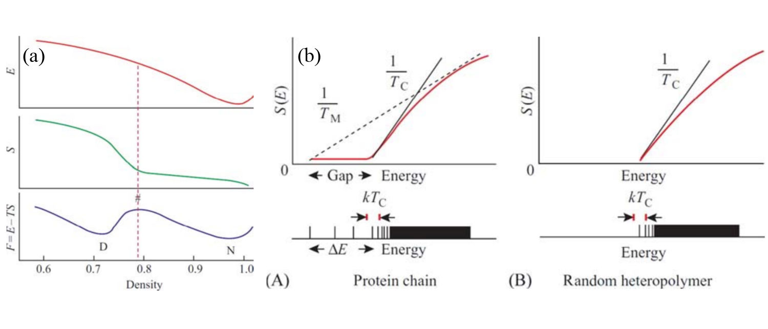
Figure 2:(a) Typical curves for the energy, entropy and free-energy of a protein as functions of the (intramolecular) density. The D and N letters mark the positions of the denatured and native states, respectively. The hash pound marks the position of the maximum of the free-energy barrier. (b) A sketch of the energy spectra (bottom panels) and associated curves (top panels) for (A) a protein and (B) a random heteropolymer. Adapted from Finkelstein & Ptitsyn (2002).
Figure 2(a) shows the origin of the “all-or-none” transition observed in protein denaturation in thermodynamic terms. Here I will use the description given by Finkelstein & Ptitsyn (2002) (whence the figure comes), almost word by word. The panel shows the energy and the entropy of a protein as a function of its internal density (in some arbitrary units). The energy is at its minimum at close packing, while the entropy S increases with decreasing density. Initially, this increase is slow, since the side chains can only vibrate, but their rotational isomerization is impossible. When the density decreases enough that the latter becomes possible the increase is much steeper. Finally, when free isomerization has been reached the entropy growth becomes slow again.
The nonuniform growth of the entropy is due to the following. The isomerization needs some vacant volume near each side group, and this volume must be at least as large as a group. And, since the side chain is attached to the rigid backbone, this vacant volume cannot appear near one side chain only but has to appear near many side chains at once. Therefore, there exists a threshold (barrier) value of the globule’s density after which the entropy starts to grow rapidly with increasing volume (decreasing density) of the globule. This density is rather high, about of the density of the native globule, since the volume of the group amounts to of the volume of an amino acid residue. Therefore, the dependence of the resulting free energy on the globule’s density has a maximum (the so-called free-energy barrier) separating the native, tightly packed globule (N) from the denatured state (D) of lower density. It is because of the presence of this free energy barrier that protein denaturation occurs as an “all-or-none” transition akin to melting or nucleation, independent of the final state of the denatured protein.
It is useful, when talking about proteins, to also introduce the concept of random heteropolymers, which are polymers with sequences that have not been selected by nature, and therefore have many (degenerate or quasi-degenerate) ground states rather than a single native conformation. Figure 2(b) shows the qualitative difference between a protein and a random heteropolymer. The bottom panels of the figure show the typical energy spectra of the two chains, where each line corresponds to a single conformation. At high energy both spectra are essentially continuous. However, the low-energy, discrete parts look very different: the energy difference between the ground state and the continuous part of the spectrum, where the majority of the “misfolded” states lie, is much larger in a protein than in a random heteropolymer. It is this energy gap that creates the free-energy barrier of Figure 2(a).
We can also define the entropy , which is proportional to the logarithm of the number of structures having energy , and the temperature corresponding to the energy , implicitly defined by the relation . As sketched in Figure 2(b), the peculiar shape of the protein energy spectrum gives raise to a concave part of , which means that there is a temperature at which the lowest-energy, native conformation coexists with many high-energy (denatured) ones. In this simple picture, this is the melting temperature . This temperature should be compared with the so-called “glass temperature” , called in the figure, which is the temperature associated to the lowest energy of the continuous band of the spectrum. Above the chain behaves, from the kinetic point of view, like a viscous liquid, while below the glass temperature the behaviour is glassy-like (i.e. non-Arrenhius dependence on temperature, aging, non ergodicity, etc.).
If , the slow dynamics asssociated to the glass state makes it kinetically impossible to reach the ground state, and the chain remains trapped in higher-energy misfolded states. By contrast, if , folding is possible, and results obtained with minimalistic models show that the fraction is a good proxy for “foldability”: the larger this fraction, the faster the protein folds.
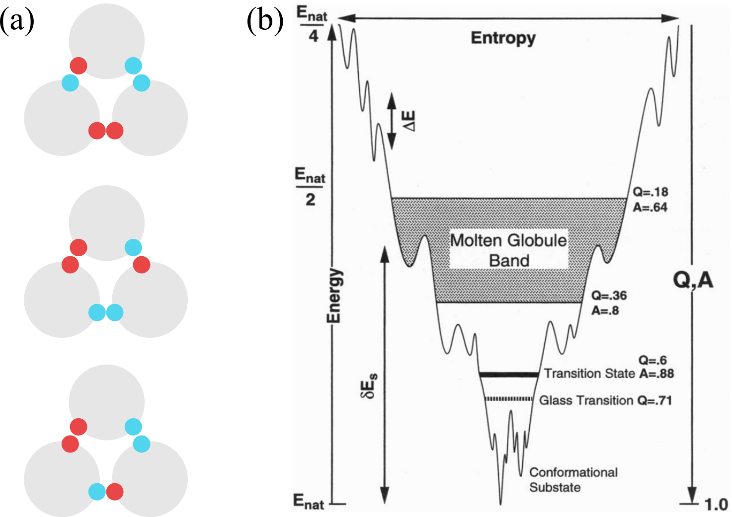
Figure 3:(a) An example of frustrated interactions: if the particle-particle interaction is such that only like colours want to be close to each other, there is no way of arranging the three spheres so that all favourable contacts are made. As a result, the ground state is degenerate. (b) A schematic energy landscape of a 60 amino-acid helical protein. and are the fractions of correct dihedral angles in the backbone and correct native-like contacts, respectively, is the “ruggedness” of the landscape, and is the energy gap. Taken from Onuchic et al. (1995).
All these concepts are not merely qualitative, but have been grounded in theory by using sophisticated statistical mechanics approaches that have generated the “funnel landscape” folding picture, which is schematically shown in Figure 3(b).
The basic idea is to leverage the concept of frustration, which happens when the interactions between the different parts of a system are such that they cannot be satisfied, from the energetic point of view, all at the same time. If this is the case, then there is no single ground state, but rather many low-energy stable states that, in a many-body system, are uncorrelated from each other and separated by (possibly large) energy barriers. An example is provided in Figure 3(a). The resulting “energy surface” (or landscape) is said to be rugged (or rough), and generates a dynamics where the system sits in a valley for a long time before being able to jump over the barrier and move to a different stable conformation. This is a hallmark of glassiness.
To draw a parallel with proteins, we can consider a random heteropolymer, where the interactions among the different amino acids will be frustrated, blocking the system from finding a single well isolated folded structure of minimum energy. A candidate principle for selecting functional sequences is thus the minimization of this frustration. Of course even in the absence of frustration, there are still energetic barriers on the path towards the native conformation due to local structural rearrangements which still give raise to a rugged landscape, slowing down the kinetics towards the folded state. This scenario has come to be called a folding “funnel”, emphasizing that there is a single dominant valley in the energy landscape, into which all initial configurations of the system will be drawn.
A classic funnel diagram, such as the one shown in Figure 3(b), represents an energy-entropy landscape, with the width being a measure of the entropy, whereas the depth represents both the energy and two correlated order parameters and , which are the fractions of native contacts and correct dihedral angles in the protein backbone. Although in reality the landscape is multidimensional, here the projection attempts to retain its main features, such as the barrier heights, which are a measure of the “ruggedness” or “roughness” of the landscape. The typical height of these barriers, together with the energy gap and the number of available conformations, are the three main parameters of the Random Energy Model, which is one of the main theoretical tools in this context.
1.1The Zimm-Bragg model for the helix-to-coil transition
As we discussed, polypeptides can, in general, be reversibly denatured (with temperature or pH, for instance). Here we theoretically investigate this phenomenon in the context of secondary structure with the Zimm-Bragg model, which is a toy model for a chain that can exhibit a continuous coil-to-helix transition. Note that it is possible to synthesise polypeptide chains that undergo such a transition, see e.g. Doty & Yang (1956).
Consider a polymer chain composed of residues. Each residue can be in one of two states, “coil” (c) or “helix” (h), so that a microscopic state of the chain can be expressed as a one-dimensional sequence, like ccchhhhhcchhhchcc. In equilibrium, the probability (or statistical weight) to observe a given chain microstate is just the Boltzmann factor, , where is the free-energy cost of the microstate, so that the total (configurational) partition function is
Since (free) energies are always defined up to a constant, we define the free-energy of a coil of any length to be zero by definition, so that the statistical weight of a coil residue is always 1. By contrast, forming a sufficiently long helical segment should be advantageous, otherwise no transition would occur. However, we know that in the helices formed by polypeptides, each -th amino acid is hydrogen-bonded to the -th, where for a -helix. As a consequence, since one full helical turn needs to be immobilised before seeing any benefit from the formation of hydrogen bonds, the formation of a helix incurs a large entropic penalty that needs to be paid every time a coil segment turns into a helical one, . However, once a helix is formed and the initial price has been paid[1], adding an H contributes a fixed amount to the helix free energy. As a result, the free-energy contribution of a helical stretch of size is , so that is statistical weight is
where we have defined the cooperativity (or initiation) parameter, , and the helix-elongation (or hydrogen-bonding) parameter, . Note that, since is purely entropic, and therefore does not depend on temperature.
Following Finkelstein & Ptitsyn (2016), we define two accessory quantities: is the partition function of a chain of size , where the last monomer is in the coil state, and is the partition function of a chain of size , where the last monomer is in the helix state. With this definition, the partition function of the chain is . We can explicitly compute the first terms:
For , the sequence is either
corh, so that and .For , we have two sequences ending with c, which are
hcandcc, and two sequences ending with h, which arehhandch. Each partition function is given by a sum of the statistical weights of the allowed microstates, so that we have and .For , there are 8 available sequences, which are built by taking each sequence and adding either
corhat its end. Each of the resulting sequence will have a statistical weight that is that of the base sequence, multiplied by 1 if the sequence ends withc, and by or if the sequence ends withhand the preceeding character ishorc, respectively. Summing up the contribution we obtain and .
In general the operations carried out to compute the partial partition functions can be applied to any other value of , meaning that we can write down recursive relationships connecting and to and . These relationships can be neatly expressed in matricial form:
It is convenient to define the matrix
so that the total partition function of a chain of monomers can be written as[2]
where the first vector-matrix multiplication on the right-hand side gives , which multiplied by the column vector yields . The partition function can be written in terms of the eigenvalues of if we note that
where , and and (with ) are the eigenvalues of , which can be found by solving the secular equation, viz.:
whence
Note that the two eigenvalues are linked by the relation .
Since they can be of any length, the two eigenvectors and of a 2x2 matrix each have a single independent element, (where ), which is given by
We obtain and , and therefore and . The two eigenvectors are used to construct the diagonalising matrix and its inverse[3]
We can now write Eq. (7) explicitly in terms of and :
From the partition function we can compute any observable we need. The most interesting quantity is the average fraction of residues that are in the helical state h, which can be compared to experiments. First of all, we note from the and we explicitly calculated and from Eq. (5) that the partition function is a polynomial in , and therefore can be written as
where are coefficients that do not depend on , but only on and on the multiplicity of each state with helical residues. Therefore, by definition the probability that the chain has exactly helical residues is , which means that the average number of helical residues is
since and only depends on . Defining the fraction of helical residues, , and exploiting the known property of logarithms we find
Substituting Eq. (13) it is possible to write in the following closed, albeit rather cumbersome, form :
For sufficiently long chains, and the expression can be greatly simplified:
The model as described and solved takes into account the cooperativity of the transition through the parameter . It is instructive to look at the non-cooperative solution, which can be obtained by setting . In this case and , so that
which is independent of and describes the simple chemical equilibrium of a reaction. Indeed, defining the equilibrium constant , where is the concentration of , we find that the fraction of residues in the helical state is
which, if compared with Eq. (19), shows that .
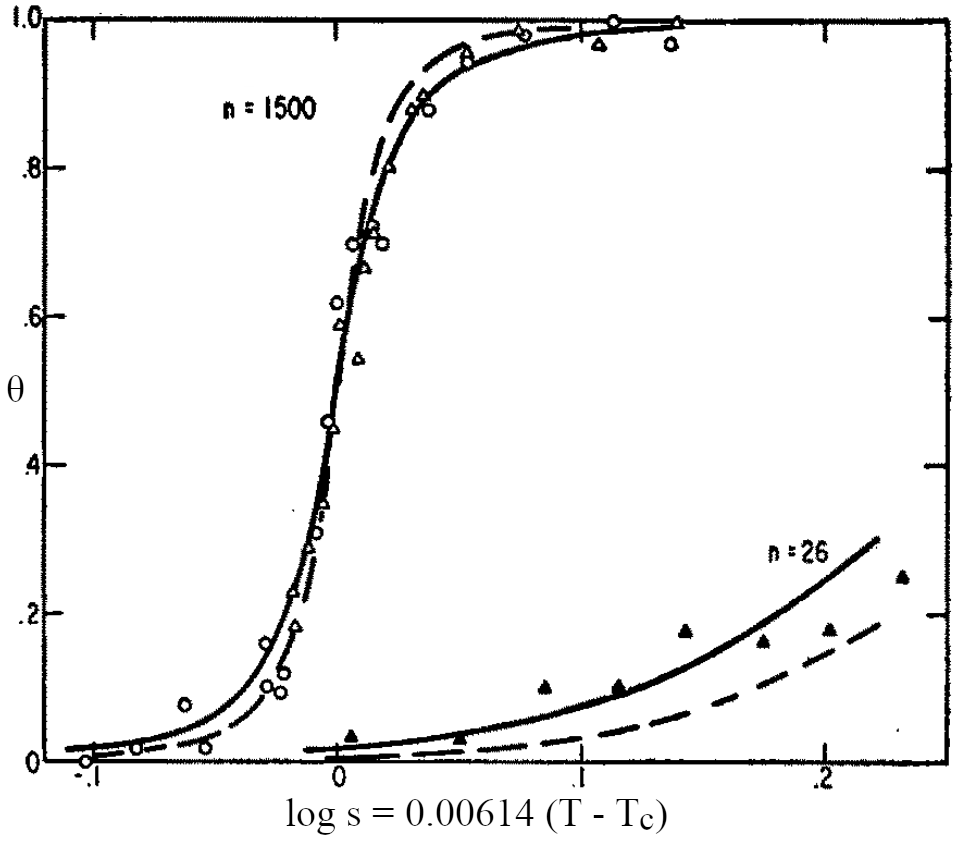
Figure 4:Comparison between experimental data (points) and theoretical fits to Eq. (17) (lines). The number of monomers is and for the top and bottom curves, respectively. is fixed by the relation , where is the temperature at which . Solid and dashed lines correspond to and , respectively. Adapted from Zimm & Bragg (1959).
A comparison between the Zimm-Bragg theory and experiments on poly--benzyl-L-glutamate of different lengths are reported in Figure 4. It is clear that there is a strong -dependence that shows the cooperative nature of the transition. Moreover, in fitting the curves it is assumed that does not depend on , since it has a purely entropic origin. However, note that in this particular experimental system the observed fraction of helical monomers grows with temperature: due to the combination of solvent and peptides used, the parameter here takes into account not only the enthalpic contribution due to the residue-residue interactions, but also the contribution due to solvent-solute interactions.
1.2The HP model
Globular proteins exhibit a unique characteristic compared to other isolated polymer molecules: their native structure is unique, meaning that the path formed by the backbone is essentially fixed, bar some small fluctuations. The question arises: what forces, determined by the amino acid sequence, contribute to this remarkable specificity? Of course, as discussed before, a significant constraint is provided by the fact that native structures are compact. However, even for compact chain molecules, many conformations are possible, with the number of maximally compact conformations increasing exponentially with chain length. Among the various physically accessible compact conformations, there are in principle many different interactions that can impact their thermodynamic stability and thus select the native structure. However, it is now well accepted that the interaction type that most contribute to this conformational reduction is hydrophobicity: given a specific amino acid sequence, the number of compact conformations that it can take is greatly reduced by the constraint that residues with hydrophobic side chains should reside inside the globule, while polar and hydrophilic residues should be on the protein’s surface (see e.g. Finkelstein & Ptitsyn (2002) and Dill (1990)).
A simple model that has been used to demonstrate the importance of hydrophobic interactions in selecting the native structure is the Hydrophobic-Polar (HP) protein lattice model. In this model, proteins are abstracted as sequences composed solely of hydrophobic (H) and polar (P) amino acids. In the HP model, the protein sequence is mapped onto a grid, or lattice, which can be two-dimensional (2D) or three-dimensional (3D). Common lattice types used include square lattices for 2D models and cubic lattices for 3D models, but other choices are possible.
Here I will present the 2D square lattice version of the model[4]. Each of the amino acids of the protein is assigned a type: “H” means hydrophobic, and “P” means polar, so that the sequence of the protein is then the ordered list of amino acids (e.g. “HHPHPPPHHP”). The -th amino acid in the sequence is identified by its index and occupies a point on this grid, and two amino acids cannot occupy the same grid point. Two amino acids and for which are “connected neighbours” and share a backbone edge representing the peptide bond, which on the square lattice can be either horizontal or vertical. By contrast, two amino acids and for which that are adjacent in space but not along the sequence are said to be “topological neighbours”. Every pair of HH topological neighbours form a topological contact that contributes an amount of free energy , while the other contacts give and . In the simplest version of the model . In this case, the total (dimensionless) free energy of a conformation is
where is the number of HH topological contacts. Following Lau & Dill (1989), the lowest-energy (highest-) conformations of a chain with a specific sequence and a length are called “native”.
The concept of topological contacts is also useful to describe the degree of compactness of a conformation, defined as
where is the number of topological contacts, irrespective of the type of neighbouring residues, and is the largest possible number of topological contacts for a chain of size , which is
where is the perimeter of the smallest box that can completely surround the protein. By this definition, (maximally) compact conformations have .
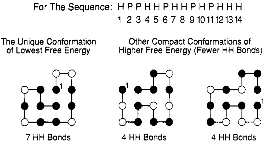
Figure 5:The sequence “HPPHHPHHPHPHHH” has a single conformation with 7 topological contacts (shown on the left). All other conformations, like the two on the right, have fewer hydrophobic contacts. Hydrophobic and polar residues are shown as black and white circles, respectively. Taken from Dill (1990).
As an example, Figure 5 shows the single lowest-energy conformation of a given sequence, together with two other compact conformations of higher free energy. It is rather evident that the native conformation has a core that is richer in hydrophobic residues compared to the other two.
In order to be more quantitative, some useful observables can be introduced. In general, the thermodynamic properties of a chain of length and a given sequence can be computed from the partition function:
where is the number of distinct conformations of an -chain, so that the sum runs over all the conformations. If the length of the chains is not too large[5], it is possible to numerically perform a complete (exhaustive) enumeration of all possible chain conformations, from which any quantity of interest can be computed as an ensemble average, viz.
Since , the partition function can also be written as a sum over conformations of fixed number of HH topological contacts :
where is the maximum number of HH topological contacts and is the number of distinct chain conformations having . Note that by this definition, the native conformations are those for which . We also define as the number of conformations that have HH topological contacts and non-HH topological contacts, which is connected to by
Since partition functions are defined up to a multiplicative constant, we multiply by to obtain[6]
With this definition it is straightforward to take averages over native conformations only. Indeed, if we take the limit, is non-zero only for , and the partition function becomes
We now define some useful average values to characterise the different states. The average compactness over all conformations is
and the average compactness over the native conformations is
where we used the fact that
The average energy is proportional to the average number of HH contacts, which is
Finally, we know already that most of the hydrophobic residues are buried in the core of globular proteins. In the HP model we define the core as the set of residues that are completely surrounded by other residues. Let the number of core residues be , and the number of hydrophobic core residues be , then the degree of hydrophobicity of a given conformation can be estimated as
and its averages over all and native conformations can be computed as
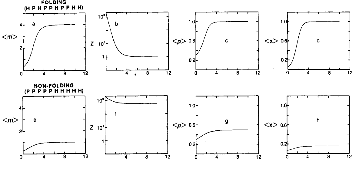
Figure 6:Ensemble averages of folding (top) and non-folding (bottom) sequences. Here is the value of the partition function, which I call . All quantities are plotted as a function of . Adapted from Lau & Dill (1989).
The ensemble averages of these quantities, as well as of the partition function, which is a measure of the number of available conformations, as a function of for two sequences are shown in Figure 6. Looking at the top panels it is clear that if the HH interaction is strong the preferred conformations of the HPHPPHPPHH sequence have low energy, are few (), compact, , and have a purely hydrophobic core, : this is a “folding” sequence.
By contrast, the bottom panels show a sequence that behaves very differently: the low-energy (native) conformations are not compact and large in number. Looking at the sequence itself, PPPPPHHHHH, it is clear that the hydrophilic “tail” does not make it possible to form a conformation with a hydrophobic core, and the number of HH topological contacts itself cannot be too high. These are all clear signs of a “non-folding” sequence.
Note that the quantities reported in Figure 6 are somewhat correlated: folding sequences tend tend to have few (sometimes one) low-energy compact conformations with hydrophobic cores, whereas non-folding sequences tend not to have any of these attributes.
The HP model (or its extensions) can be used to understand some general or even specific aspects of protein folding because of its simplicity. The 2-letter alphabet and the greatly reduced residue conformations due to the underlying lattice makes it possible to fully explore (at the same time) the conformational space (i.e. the set of all possible internal conformations of a molecule) and the sequence space (i.e. the set of all possible sequences of H and P residues). Both spaces have sizes that grow exponentially with , and therefore the maximum length of chains that can be investigated by exhaustive enumeration is somewhat limited, but there are computational techniques that can be used to circumvent this issue.
1.2.1Folding HP sequences
If we now use a stricter definition of a “folding” sequence as a sequence that has a single native conformation, we can draw a comparison between lattice folding sequences and real proteins. First of all, how many folding sequences there are?
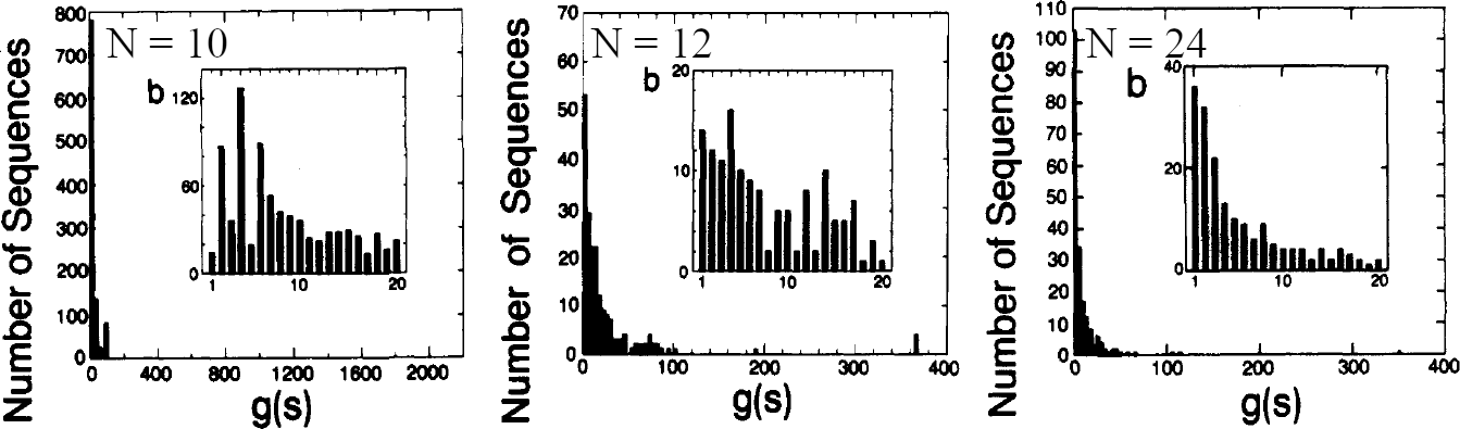
Figure 7:The distribution of the number of sequences having native conformations for chain length and 24. In the figure . Adapted from Lau & Dill (1989).
Figure 7 shows the distributions of the number of native conformations , i.e. how many sequences have the given degeneracy, for different chain lengths. As increases, the distribution becomes more and more peaked on 1: far more sequences have a single lowest-energy conformation rather than, say, 10 or 100. These results suggest that hydrophobicity alone is enough to greatly reduce the number of compact configurations into a small set of folding candidate structures (Dill (1990)), and confirms that the hydrophobic force is a major driving force for protein folding (see e.g. Finkelstein & Ptitsyn (2002)).
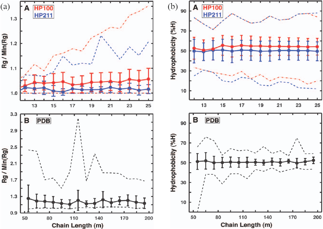
Figure 8:(a) Compactness and (b) hydrophobicity as a function of the chain length for (A) two HP lattice models and (B) real proteins. Dashed lines show the range of values. Adapted from Moreno‐Hernández & Levitt (2012).
But to what extent lattice and real proteins are similar? I will present some results reported in Moreno‐Hernández & Levitt (2012). Therein, an exhaustive enumeration of all conformations of chains of lengths up to 25 has been carried out with two HP models:
In HP100, which is the one described above, only HH contacts contribute to a conformation’s free energy.
In HP211 topological contacts between H and P and P and P contribute -1 (i.e. ) to the free energy, while HH contacts contribute . As a result, compared to the HP100 model, all residues feel an attraction that makes compact conformations more favourable.
Some interesting results pertaining to folding sequences are reported in Figure 8. Figure 8(a) shows, as a proxy for compactness, the normalised radius of gyration , where is the smallest radius of gyration among the structures of a given length, for the lattice and real proteins. For real proteins the authors have considered a non-redundant set of 2401 single-domain proteins from the PDB with lengths between 50 and 200 residues long. By comparing the two lattice models, it is evident that the additional attraction between non-hydrophobic residues enhances the compactness in HP211 more, but the variation in compactness, given by the error bars, is very small in both cases, and the compactness itself does not depend on the chain length. The same behaviour is observed in real proteins.
Figure 8(b) shows the percentage of residues that are hydrophobic in the lattice structures and for the same real proteins used for the radius of gyration. Both lattice and real proteins have an average hydrophobicity of , independent of , and the error bars and total range (dashed lines) are comparable in the two cases (although both are a bit larger for the HP model). Folding sequences in the HP model are “protein-like”.
1.2.2Designable HP conformations
Now we focus on compact conformations. How many sequences have a given compact conformation as their native (i.e. lowest-energy) state? Does the answer depend on some properties of the selected conformation itself? In the context of the HP model, some of the first answers were provided here with a HP model with , and , chosen in order to fulfill the following physical constraints, rooted in the analysis of real proteins:
Compact conformations have lower energies compared to non-compact ones.
Hydrophobic residues should have the tendency to be buried in the core ().
Different types of monomers should tend to segregate ().
The output of the computation was to enumerate all the native structures of each possible sequence on a 3D 3x3x3 cube and on 2D 4x4, 5x5, 6x5 and 6x6 boxes. The result of this complete enumeration is the list of all possible sequences that can “design” a given structure, or, in other words, that have that structure as their unique native state. The size of this list, , is a measure of the designability of a given structure.
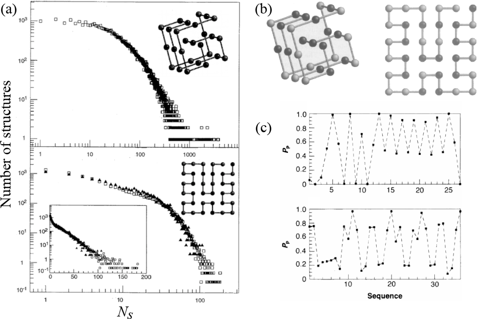
Figure 9:(a) The number of structures with the given for the (top) 3x3x3 cube and (bottom) 6x6 square. In the bottom panel, the number of structures goes below 1 for large , which, given its definition, should not happen. Perhaps the authors normalised the data in some way that, as far as I understand, is not specified in the original paper. (b) The most designable (A) 3D and (B) 2D structures. Hydrophobic and polar residues are coloured in black and grey, respectively. (c) The probability of finding a polar residue as a function of the sequence index for the same two structures. Adapted from Li et al. (1996).
Compact structures differ markedly in terms of their designability: there are structures that can be designed by a large number of sequences, and there are “poor” structures that can be designed by only a few or even no sequences. In fact, for of the conformations there is no sequence that has that structure as its ground state. The majority of the sequences ( out of the 227 total sequences in 3D) have degenerate ground states, i.e. more than one compact conformation of lowest energy, which means that in 3D there exist almost 7 million sequences of length 27 that have a unique compact ground state. Moreover, the number of structures with a given value decreases continuously and monotonically as increases. The data for the 3D and largest 2D cases is shown in Figure 9(a), where the long tails of the distributions, with some structures being the ground states of thousands of sequences, highlight the presence of “highly-designable” compact conformations.
Structures with large exhibit specific motifs (i.e. secondary structures) that small compact structures lack. For instance, the 3D compact structures with the 10 largest values contain parallel running lines packed regularly and eight or nine strands (three amino acids in a row), sensibly more than the average compact structure. Figure 9(b) shows the most designable structures in 3D and in 2D, where it is easy to spot the regularity of the “secondary structures” and, for the 3D structure, also the “strands”.
With the simple lattice model is also possible to directly assess the effect of mutations, which in real proteins is particularly important in the context of homologous sequences (sequences related by a common ancestor). Indeed, focussing on highly designable structures and referring to the different sequences that fold into them as “homologous”, it is possible to observe phenomena that are qualitatively similar to those observed in real proteins. For example, sequences that differ by more than half of their residues can design the same structure (see Figure 20, which will be discussed later, for a real-protein example). Looking at the effect of mutations, the rightmost panel of Figure 9(c) shows that in very designable conformations some residues are highly mutable, whereas others are highly conserved, with the conserved sites being those sites with the smallest or largest number of sides exposed to water.

Figure 10:The average energy gap between the lowest-energy and first excited states of the (a) 3D 3x3 cube and (b) 2D 6x6 HP models, as well as of the (c) 2D 6x6 MJ model. Adapted from Helling et al. (2001)).
Another important feature of proteins that is also reproduced by the model is the large energy gap between the lowest-energy and first excited conformations, which stabilises the native structures from the thermodynamic point of view. In the lattice model, the average energy gap is defined as the minimum energy required to change a native conformation to a different compact structure, averaged over all the sequences that design that native conformation. Figure 10 shows that there is a sudden jump (in 3D) or change of slope (in 2D) at a specific value of . Therefore, the conformations that are highly designable also have large energy gaps, making them highly stable from a thermodynamic point of view.
As shown in the rightmost panel of Figure 10, the same behaviour is also observed when a 20-letter (rather than 2-letter) alphabet is used, with the interactions between the residues being modelled using the MJ interaction matrix, which was derived by analysing the contact frequencies of amino acids from protein crystal structures.
Although the ingredients in the simple lattice model are minimal, lacking many of the factors that contribute to the structure of proteins, the results that have been obtained with it contributed to the understanding that there is a link between designability and thermodynamic stability: “From an evolutionary point of view, highly designable structures are more likely to have been chosen through random selection of sequences in the primordial age, and they are stable against mutations” (Li et al. (1996)).
1.3Sequence alignment
Simple models are useful to understand the underlying physics of some particular phenomena. However, how can we understand something very specific, like what is the 3D structure of a particular sequence? The simplest way is to look for similarities: if we already have a list of sequence structure connections, we can try to look whether the new sequence, for which the 3D structure is unknown, is similar, and to what degree, to another for which the 3D structure is already known. This operation is called “sequence alignment” (SA).
Sequence alignment is a fundamental technique in bioinformatics. The primary goal of sequence alignment is to identify regions of similarity that may indicate functional, structural, or evolutionary relationships between the sequences being compared. In the context of proteins, sequence alignment can be useful for reasons that go beyond the 3D structure prediction:
It helps to predict the function of unknown proteins based on their similarity to known proteins.
It aids in understanding evolutionary relationships by identifying conserved sequences among different species, allowing the construction of phylogenetic trees.
It can identify conserved domains that are crucial for the function of proteins.
It helps in identifying potential drug targets by finding unique sequences in pathogens that differ from the host.
It assists in annotating genomes by finding homologous sequences, thus providing insights into gene function and regulation.
Turning a biological problem into an algorithm that can be solved on a computer requires making some assumptions in order to obtain a model with relative simplicity and tractability. In practice, for our sequence alignment model we ignore realistic events that occur with low probability (e.g. duplications) and focus on the following three mechanisms through which sequences vary:
A (point) mutation, or substitution, occurs when some amino acid in a sequence changes to some other amino acid during the course of evolution.
A deletion occurs when an amino acid is deleted from a sequence during the course of evolution.
An insertion occurs when an amino acid is added to a sequence during the course of evolution.
There are many possible sequences of events that could change one genome into another, and we wish to establish an optimality criterion that allows us to pick the “best” series of events describing changes between sequences. We choose to invoke Occam’s razor and select a maximum parsimony method as our optimality criterion[7]: we wish to minimize the number of events used to explain the differences between two sequences. In practice, it is found that point mutations are more likely to occur than insertions and deletions, and certain mutations are more likely than others. We now develop an algorithmic framework where these concepts can be incorporated explicitly by introducing parameters that take into account the “biological cost” of each of these changes.
1.3.1Homology
While here my focus is on protein structure, I also want to point out that in bioinformatics one of the key goals of sequence alignment is to identify homologous sequences (e.g., genes) in a genome. Two sequences that are homologous are evolutionarily related, specifically by descent from a common ancestor. The two primary types of homologs are orthologous and paralogous. While they are outside the scope of these notes, I note here that other forms of homology exist (e.g., xenologs, which are genes in different species that have arisen through horizontal gene transfer[8] rather than through vertical inheritance from a common ancestor, and often perform similar functions in their respective organisms despite their distinct evolutionary origins).
Orthologs arise from speciation events, leading to two organisms with a copy of the same gene. For example, when a single species A speciates into two species B and C, there are genes in species B and C that descend from a common gene in species A, and these genes in B and C are orthologous (the genes continue to evolve independent of each other, but still perform the same relative function).
Paralogs arise from duplication events within a species. For example, when a gene duplication occurs in some species A, the species has an original gene B and a gene copy B’, and the genes B and B’ are paralogus.
Generally, orthologous sequences between two species will be more closely related to each other than paralogous sequences. This occurs because orthologous typically (although not always) preserve function over time, whereas paralogous often change over time, for example by specializing a gene’s (sub)function or by evolving a new function. As a result, determining orthologous sequences is generally more important than identifying paralogous sequences when gauging evolutionary relatedness.
1.3.2Definitions
Following Kellis (2016), we introduce a simplified version of the alignment problem and make it more complex by adding the required ingredients. First, some definitions:
- Sequence
- In mathematics (and combinatorics) a sequence is a series of characters taken from an alphabet . For what concerns us, DNA molecules are sequences over the alphabet , RNA sequences over the alphabet , and proteins are sequences over the alphabet .
- Substring
- A consecutive part of a sequence. A sequence of length has substrings of length 1, substrings of length 2, , 2 substrings of length . Given the sequence “SUPERCALIFRAGILISTICHESPIRALIDOSO”, “FRAGILI” is a substring, but “SUPERDOSO” is not.
- Subsequence
- A set of characters of a sequence. The characters do not have to be consecutive, but they should be ordered like in the original sequence. Given the sequence “SUPERCALIFRAGILISTICHESPIRALIDOSO”, “FRAGILI” and “SUPERDOSO” are two subsequences, but “SOSUPER” is not. Formally, given a sequence , , with , is a subsequence of if there exists a strictly increasing sequence of indices of such that for each .
- Sequence alignment
- An alignment of two sequences and , defined over the same alphabet , is a table containing either a character from , or the gap symbol “
-”. In the table there is no column in which both characters are “-”, and the non-gap characters in the first line give back sequence , while the non-gap characters in the second line give back sequence .
1.3.3Problem formulation
We warm up by considering the following simple problem: given two sequences, and , what is their longest common substring? We take the two following DNA fragments as examples: ACGTCATCA and TAGTGTCA. The problem can be solved by aligning the first characters of the two sequences, and then shifting one, say , by an integer amount . By computing the number of matching characters for every we can find the optimal alignment, which in this case is given by :
--ACGTCATCA
--xx||||---
TAGTGTCA---
The first and third rows of the diagram above describe the alignment itself, as introduced earlier, showing that gaps are characters that align to a space, while the central row shows the character matches: here x and | stand for mismatches and matches, respectively. In this example, the longest common substring is GTCA. The algorithm I just described has a complexity of , where is the length of the shortest sequence.
A more complicated problem is to find the longest common subsequence (LCS) between two sequences. In the language we are introducing, this means allowing internal gaps in the alignment. The LCS between the and sequences defined earlier is
-ACGTCATCA
-|-||x-|||
TA-GTG-TCA
In this case the LCS is AGTTCA, which is longer than the longest common substring.
The LCS problem as formulated here is a particular case of the full sequence-alignment problem. In order to generalise the problem, we introduce a cost function that makes it possible to recast it in terms of an optimisation problem. Given two sequences and , we define as the “biological cost” of turning into . For the case just considered, I implicitly used as a cost function the Levenshtein (or edit) distance, which is defined as the minimum number of single-character edits required to change one string into another. In other words, the problem has been formulated by implicitly considering that all possible operations (mutations, insertions and deletions) are equally likely. In a more generalised formulation, each edit operation is associated to a specific cost (penalty) that should reflect its biological occurrence, as discussed later.
What about gaps? In general, the cost of creating a gap depends on many variables. There are varying degrees of approximations that can be taken in order to simplify the problem. At the zero-th order each gap can be assumed to have a fixed cost, as we implicitly did above. This is called the “linear gap penalty”. An improvement can be done by considering that, biologically, the cost of creating a gap is more expensive than the cost of extending an already created gap. This is taken into account by the “affine gap penalty” method, whereby there is a large initial cost for opening a gap, and then a small incremental cost for each gap extension. There are other (more complicated and more context-specific) methods that can be considered and that we will not analyse further here, such as the general gap penalty, which allows for any cost function, and the frame-aware gap penalty, which is applied to DNA sequences and tailors the cost function to take into account disruptions to the coding frame[9].
1.3.4The Needleman-Wunsch algorithm
Once we allow for gaps, the enumeration of all possible alignments (as done for the longest common substring method) becomes unfeasible. Indeed, the number of non-boring alignments, i.e. alignments where gaps are always paired with characters, in a sequence of size containing gaps (where ) can be estimated as
where we used the second-order Stirling’s approximation, . Note that this number grows very fast: for it is already larger than 1017. Considering that we also have to compute the score of each alignment, it is clear that the problem is untractacle with a brute-force method. Here is where dynamic programming enters the field.
Suppose we have an optimal alignment for two sequences , of length , and , of length , in which matches . The alignment can be conceptually split into three parts:
Left subalignment: The alignment of the subsequences
and . Middle match/mismatch: The alignment of
with (this could be a match or a mismatch). Right subalignment: The alignment of the subsequences
and .
The overall alignment score is the sum of the scores from these three parts: the score of the left subalignment, the score for aligning
Let be the score of the optimal alignment of and . Since and , the matrix storing the solutions (i.e. optimal scores) of the subproblems has a size of .
We can compute the optimal solution for a subproblem by making a locally optimal choice based on the results from the smaller subproblems. Thus, we need to establish a recursive function that shows how the solution to a given problem depends on its subproblems and can be used to fill up the matrix . At each iteration we consider the four possibilities (insert, delete, substitute, match), and evaluate each of them based on the results we have computed for smaller subproblems.
We start by considering the linear gap penalty model, and define , with , as the cost of a gap. We are now equipped to set the values of the elements of the matrix. Let’s consider the first row: the value of is the cost of aligning a sequence of length 0 (taken from ) to a sequence of length (taken from ), which can be obtained only by adding gaps, yielding . Likewise, for the first column we have . Then, we traverse the matrix element by element. Let’s consider a generic element : this is the cost of aligning the first characters of to the first characters of . There are three ways we can obtain this alignment:
Align to a gap (i.e. a gap is added to ): the total cost is ;
Align to a gap (i.e. a gap is added to ): the total cost is ;
and are matched: the total cost is , where is the cost of (mis)matching and .
Leveraging the cut-and-paste argument sketched above, the optimal cost is given by the largest of the three values. Formally,
This is a recursive relation: computing the value of any requires the knowledge of the values of its left, top, and top-left neighbours. Therefore, the fill-in phase amounts to traversing the table in row or column major order, or even diagonally from the top left cell to the bottom right cell. After traversing the matrix, the optimal score for the alignment is given by the bottom-right element, . In order to obtain the actual alignment we have to traceback through the choices made during the fill-in phase. It is helpful to maintain a pointer for each cell while filling up the table that shows which choice was made to get the score for that cell. Then the pointers can be followed backwards to reconstruct the optimal alignment.
The complexity analysis of this algorithm is straightforward. Each update takes time, and since there are elements in the matrix , the total running time is . Similarly, the total storage space is . For the more general case where the update rule is more complicated, the running time may be more expensive. For instance, if the update rule requires testing all sizes of gaps (e.g. the cost of a gap is not linear), then the running time would be ).
1.3.5Local alignment: the Smith-Waterman algorithm
The Needleman-Wunsch algorithm finds the best possible alignment across the entire length of two sequences. It tries to align every character from the start to the end of the sequences, which means both sequences are considered in their entirety. This is called “global alignment”, and it is most useful when the sequences being compared are of similar length and are expected to be homologous across their entire length.
Local alignment, on the other hand, focuses on finding the best alignment within a subset of the sequences. It identifies regions of similarity between the two sequences and aligns only those regions, ignoring the parts of the sequences that do not match well. Local alignment is particularly useful when comparing sequences that may only share a segment of similarity, such as when comparing domains within proteins, detecting conserved motifs, or identifying homologous regions in sequences that may not be overall similar[10], which is why it is very useful for the prediction of the 3D structure of proteins (or protein subdomains).
The most used method for local alignment is the Smith-Waterman algorithm, which is a modification of the Needleman-Wunsch algorithm. The key difference between the two lies in how the scoring matrices are constructed and scored. In Needleman-Wunsch, every cell in the matrix is filled to reflect the best global alignment, with the final alignment score found in the bottom-right corner of the matrix. Smith-Waterman, on the other hand, sets any negative scores to zero, which allows the algorithm to “reset” when the alignment quality dips. The highest score in the matrix indicates the end of the best local alignment, which is then traced back to a zero to identify the optimal aligned subsequence. This approach ensures that only the most relevant, highest-scoring local alignments are highlighted. Here is how the Smith-Waterman algorithm looks like in practice:
Initialisation: since a local alignment can start anywhere, the first row and column in the matrix are set to zeros, i.e. , .
Iteration : this step is modified so that the score is never allowed to become negative but it is reset to zero. This is done by slightly modifying Eq. (37) as follows:
Trace-back: starts from the position of the maximal number in the table and proceeds until a zero is encountered.
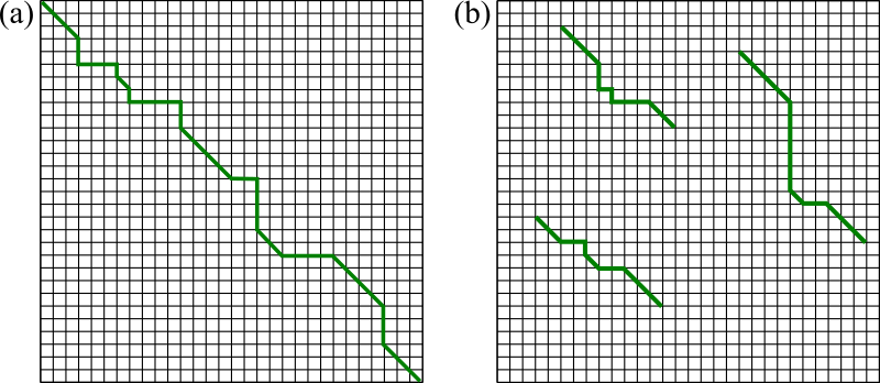
Figure 12:Example trace-back solutions generated by (a) global and (b) local alignment methods.
A visual comparison between the tables generated by global and local alignment algorithms is shown in Figure 12.
1.3.6Affine gap penalty
For both the global and local alignment algorithms introduced we have used a linear gap penalty: the cost of adding a gap is constant, regardless of the nature of the aligned character, or of the length of the gap. From the biological point of view, this means that an indel of any length is considered as the result of independent insertions or deletions. However, in reality long indels can form in single evolutionary steps, and in these cases the linear gap model overestimates their cost. To overcome this issue, more complex gap penalty functions have been introduced. As mentioned before, a generic gap penalty function would result in an algorithmic complexity worse than (where for simplicity I’m considering two sequences of the same length). Let’s see why. Any gap penalty function can be implemented in the Needleman-Wunsch or Smith-Waterman algorithms by changing the recursive rule, which can be done trivially for element by evaluating terms such as and , where is the cost of a gap of size . However, this means that the update of every cell of the dynamic programming matrix would take instead of , bringing the algorithmic complexity up to (for sequences).
However, the computational cost can be mitigated by using particular gap penalty functions. Here I will present the most common variant, which is known as the affine gap penalty. In this model, the cost of a gap of size is
where and are the opening and extension penalties, respectively, and . To incorporate affine-gap penalties into the Needleman-Wunsch or Smith-Waterman algorithms in an efficient manner, the primary adjustment involves tracking whether consecutive gaps occur in the alignment. This requires the alignment process to be split into three distinct cases: insertions, deletions, and matches/mismatches. Instead of using a single dynamic programming table as in the linear-gap penalty approach, three separate tables are used: for insertions, for deletions, and for the overall score.
In this setup, each entry in the table, denoted by , stores the best alignment score when the last column includes an insertion (i.e. a gap in the first sequence), and each entry in the table, , captures the best score for alignments ending in a deletion (i.e. a gap in the second sequence). As before, records the overall score. The recursive update rules of the three tables are
Note that with this algorithm each cell update is , and therefore the overall complexity remains the same ( or for same-length sequences).
1.3.7Substitution matrices
How is the substitution matrix determined? One possibility is to leverage what we know about the biological processes that underlie mutations. For instance, in DNA the biological reasoning behind the scoring decision can be linked to the probabilities of bases being transcribed incorrectly during polymerization. We already know that of the four nucleotide bases, A and G are purines, while C and T are pyrimidines. Thus, DNA polymerase is much more likely to confuse two purines or two pyrimidines since they are similar in structure. As a result, a simple improvement over the uniform cost function used above is the following scoring matrix for matches and mismatches:
| A | G | T | C | |
|---|---|---|---|---|
| A | +1 | -0.5 | -1 | -1 |
| G | -0.5 | +1 | -1 | -1 |
| T | -1 | -1 | +1 | -0.5 |
| C | -1 | -1 | -0.5 | +1 |
Here a mismatch between like-nucleotides (e.g. A and G) is less expensive than one between unlike nucleotides (e.g. T and C).
However, we can be more quantitative by taking a probabilistic approach. Here I will describe how the widely-used BLOSUM matrices are built (see also the original paper). We assume that the alignment score reflects the probability that two similar sequences are homologous. Thus, given two sequences and of the same length[11] for which we have an ungapped alingment, we define two hypotheses:
The alignment between the two sequences is due to chance and the sequences are, in fact, unrelated.
The alignment is due to common ancestry and the sequences are actually related.
Under the rather strict assumption (“biologically dubious, but mathematically convenient”, as aptly put in Eddy (2004)) that pairs of aligned residues are statistically independent of each other, so that the likelihoods associated to the two hypotheses, and , can be expressed as products of probabilities, viz.
where is the likelihood that residues and are aligned because correlated, while the product is the likelihood that the two residues are there by chance: their occurrence is unrelated and therefore the likelihood factorises in two terms that account for the average probability of observing those two residues in any protein.
In order to compare two hypotheses, a good score is given by the logarithm of the ratio of their likelihoods (the so-called log-odds score). Therefore, for our case the alignment score is
so that, thanks to the properties of logarithms and probabilities, the overall alignment score is the sum of the log-scores of the individual residue pairs. Considering 20 amino acids, there are 400 such log-scores, which form a 20x20 substitution (score) matrix. Each entry of the matrix takes the form
where is an overall scaling factor that is used to obtain values that can be rounded off to integers. Note that the previous definition can be formally substantiated (see e.g. Karlin & Altschul (1990)).
If (and therefore is positive), the substitution , and therefore their alignment in homologous sequences, occurs more frequently than would be expected by chance, suggesting that this substitution is favored in evolution. These substitutions are called “conservative”. As noted in Eddy (2004), this definition is purely statistical and has nothing directly to do with amino acid structure or biochemistry. Likewise, substitutions with , and therefore negative values of , are termed “nonconservative”.
The procedure applied to compute the and values starts with a collection of protein sequences.
The sequences are grouped into families based on their evolutionary relatedness. A common source for these families is the BLOCKS database, which contains aligned, ungapped regions of proteins that are highly conserved across members of the family.
Within these protein families, highly conserved regions (blocks) are identified. These regions are short segments of amino acid sequences that are believed to be important for the protein’s function and are conserved across different species.
Once blocks are identified, the sequences within each block are clustered, choosing a threshold value : two sequences that share more than this percentage of identical amino acids identity are clustered together, and only one representative from each cluster is used to avoid over-representation of very similar sequences.
Within each block, the actual counts of amino acid pairs are made.
The background frequencies are estimated by computing the overall frequency of each amino acid in the sequences, not considering any substitutions.
To evaluate the terms, for each position in the aligned block, we count how many times one amino acid (say, Alanine) is substituted by another amino acid (say, Glycine) in the aligned positions across the different sequences. For instance, if there is an alignment of 5 sequences, for each single position we make comparisons.
Of course, the final scores depend on : if is large, protein blocks that are still rather similar will be considered belonging to different clusters, and therefore compared to each other to derive the scores; the resulting matrix will be more sensitive in identifying closely related sequences but less effective for more distantly related sequences (and vice versa for small values of ). Common values for are , , and , which yield the matrices BLOSUM45, BLOSUM62, and BLOSUM80, with BLOSUM62 being the de-facto standard (and default) one.

Figure 13:The BLOSUM62 matrix. The amino acids are grouped and coloured based on Margaret Dayhoff’s classification. Non-negative values are highlighted. Credits to Ppgardne via Wikimedia Commons.
The BLOSUM62 matrix is shown in Figure 13. First of all, note that substitution matrices are symmetric, because the biological process of amino acid substitution is symmetric: as empirically observed, there is no preferred direction when one amino acid replaces another. Secondly, it is evident that conservative substitutions tend to be those between amino acids that are similar, as made evident by grouping the amino acids according to the classification introduced by Margaret Dayhoff.
Why the values of the matrix diagonal, representing the scores of “substituting” one amino acid with itself, are all different?
The rarer the amino acid is, the more surprising it would be to see two of them align together by chance. In the homologous alignment data that BLOSUM62 was trained on, leucine/leucine (L/L) pairs were in fact more common than tryptophan/tryptophan (W/W) pairs (, ), but tryptophan is a much rarer amino acid (, ). Run those numbers (with BLOSUM62’s original ) and you get +3.8 for L/L and +10.5 for W/W, which were rounded to +4 and +11.
1.3.8BLAST
The sheer volume of sequence data generated by modern-day high-throughput sequencing technologies presents a significant challenge. Databases now contain millions of nucleotide and protein sequences, each potentially spanning thousands of characters. When comparing a new sequence against these massive databases, traditional pairwise alignment methods like the ones we just discussed become computationally demanding. Indeed, performing a global or even local alignment between a query sequence and every sequence in a large database can require huge computational resources and time, especially as the number of sequences and their lengths continue to grow exponentially.
The need for a more efficient method resulted in the most cited paper of the 1990s, where BLAST (Basic Local Alignment Search Tool), now a critical tool in bioinformatics, was introduced. BLAST operates by finding regions of local similarity between sequences, which is more computationally feasible and faster than aligning entire sequences globally. The algorithm requires a query sequence and a target database. First of all, the query sequence is broken down into smaller fragments (called words or -mers). For each -mer, a list of similar words is generated, and only those with a similarity measure that is higher than a threshold are retained add added to the final -mer list. The similarity is evaluated by using a substitution matrix (BLOSUM62 is a common choice). Then, the target database is searched for matches to these words, extending the matches in both directions to find the best local alignments. BLAST assigns scores to these alignments based on the degree of similarity via a Smith-Waterman algorithm, with higher scores indicating closer matches.
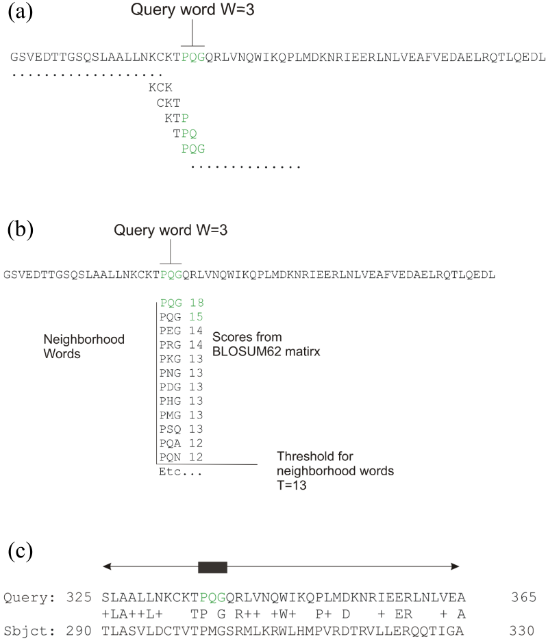
Figure 14:The three most important steps of the BLAST algorithm. (a) Generate the initial -mers (). (b) Make the list of BLAST words using a threshold . (c) Extend the matches into both directions until the score drops below a predetermined threshold.
The BLAST algorithm can be broken down into the following steps[12]
Optional: remove low-complexity region or sequence repeats in the query sequence. Here “Low-complexity region” means a region of a sequence composed of few kinds of elements. These regions might give high scores that confuse the program to find the actual significant sequences in the database, so they should be filtered out. The regions will be marked with an X (protein sequences) or N (nucleic acid sequences) and then be ignored by the BLAST program. To filter out the low-complexity regions, the SEG program is used for protein sequences and the program DUST is used for DNA sequences. On the other hand, the program XNU is used to mask off the tandem repeats in protein sequences.
Make a -letter word list of the query sequence. The words of length (-mers) in the query sequence are listed “sequentially”, until the last letter of the query sequence is included. The method is illustrated in Figure 14(a). is usually 3 and 11 for a protein and a DNA sequence, respectively.
List the possible matching words. A substitution matrix (e.g. BLOSUM62) is used to match the words listed in step 2 with all the -mers. For example, the score obtained by comparing PQG with PEG and PQA is respectively 15 and 12 with the BLOSUM62 matrix[13]. After that, a neighborhood word score threshold is used to reduce the number of possible matching words. The words whose scores are greater than the threshold T will remain in the possible matching words list, while those with lower scores will be discarded. For example, if PEG is kept, but PQA is abandoned.
Organize the remaining high-scoring words into an efficient search tree. This allows the program to rapidly compare the high-scoring words to the database sequences.
Repeat step 3 to 4 for each -mer in the query sequence.
Scan the database sequences for exact matches with the remaining high-scoring words. The BLAST program scans the database sequences for the remaining high-scoring words, such as PEG. If an exact match is found, this match is used to seed a possible ungapped alignment between the query and database sequences.
Extend the exact matches to high-scoring segment pair (HSP). The original version of BLAST stretches a longer alignment between the query and the database sequence in the left and right directions, from the position where the exact match occurred. The extension does not stop until the accumulated total score of the HSP begins to decrease. To save more time, a newer version of BLAST, called BLAST2 or gapped BLAST, has been developed. BLAST2 adopts a lower neighborhood word score threshold to maintain the same level of sensitivity for detecting sequence similarity. Therefore, the list of possible matching words list in step 3 becomes longer. Next, exact matched regions that are within distance from each other on the same diagonal are joined as a longer new region. Finally, the new regions are then extended by the same method as in the original version of BLAST, and the scores for each HSP of the extended regions are created by using a substitution matrix as before.
List all of the HSPs in the database whose score is high enough to be considered. All the HSPs whose scores are greater than the empirically determined cutoff score are listed. By examining the distribution of the alignment scores modeled by comparing random sequences, a cutoff score can be determined such that its value is large enough to guarantee the significance of the remaining HSPs.
Evaluate the significance of the HSP score. Karlin & Altschul (1990) showed that the distribution of Smith-Waterman local alignment scores between two random sequences is
where and are the length of the query and database sequences[14], and the statistical parameters and depend upon the substitution matrix, gap penalties, and sequence composition (the letter frequencies) and are estimated by fitting the distribution of the ungapped local alignment scores of the query sequence and of a lot of (globally or locally) shuffled versions of a database sequence. Note that the validity of this distribution, known as the Gumbel extreme value distribution (EVD), has not been proven for local alignments containing gaps yet, but there is strong evidence that it works also for those cases. The expect score of a database match is the number of times that an unrelated database sequence would obtain a score higher than by chance. The expectation obtained in a search for a database of total length
This expectation or expect value (often called -score, -value or -value) assessing the significance of the HSP score for ungapped local alignment is reported in the BLAST results. The relation above is different if individual HSPs are combined, such as when producing gapped alignments (described below), due to the variation of the statistical parameters.
Make two or more HSP regions into a longer alignment. Sometimes, two or more HSP regions in one database sequence can be made into a longer alignment. This provides additional evidence of the relation between the query and database sequence. There are two methods, the Poisson method and the sum-of-scores method, to compare the significance of the newly combined HSP regions. Suppose that there are two combined HSP regions with the pairs of scores and , respectively. The Poisson method gives more significance to the set with the maximal lower score . However, the sum-of-scores method prefers the first set, because is greater than . The original BLAST uses the Poisson method; BLAST2 uses the sum-of scores method.
Show the gapped Smith-Waterman local alignments of the query and each of the matched database sequences. The original BLAST algorithm only generates ungapped alignments including the initially found HSPs individually, even when there is more than one HSP found in one database sequence. By contrast, BLAST2 produces a single alignment with gaps that can include all of the initially found HSP regions. Note that the computation of the score and its corresponding -value involves use of adequate gap penalties.
The -value is the single most important parameter to rate the quality of the alignments reported by BLAST. For instance, if for a particular alignment with score , it means that there are 10 alignments with score that can happen by chance between any query sequence and the database used for the search. Therefore, this particular alignment is most likely not very significant. By contrast, values much smaller than 1 (e.g 10-3 or even smaller) are likely to signal that the sequences are homologous. On most webserver, it is possible to filter out all matches that have an -value larger than some threshold. For instance, on the NCBI webserver, the “expect threshold” defaults to 0.05.
Note that the sequence database used to search for matches is preprocessed first, which increases further the overall computational efficiency. With BLAST, the algorithmic complexity of searching the database for a sequence of length is only . An online webserver[15] to run BLAST can be found here.
1.3.9Multiple sequence alignment
Pairwise sequence alignment suffers from some issues that are intrinsic to it, and becomes glaring when trying to align sequences that are distantly related. In particular, all pairwise methods depend in some way or another on a number of parameters (scoring matrix, gap penalties, etc.), and it is hard to tell what is the “best” alignment if the method finds multiple alignments with the same score. Moreover, a pairwise alignment is not necessarily informative about the evolutionary relationship (and therefore about possibly conserved amino acids or whole motifs) of the sequences that are compared.
In order to overcome these issues, a number of multiple sequence alignment (MSA) methods have been developed. MSA extends the concept of pairwise protein alignment to simultaneously align three or more sequences, providing a broader view of evolutionary relationships, structural conservation, and functional regions among a group of proteins. Aligning multiple sequences make it possible to identify conserved amino acids that may be critical for protein function or stability and therefore are biologically significant. This, in turn, can help to predict structural features, functional motifs, and evolutionary patterns across species, providing a fundamental tool to build phylogenetic trees or inform the classification of proteins into families.
In principle, MSA can be carried out with the dynamic programming algorithms we already introduced. For instance, the recursive rule of the Needleman-Wunsch algorithm for globally aligning three sequences , , and , which extends Eq. (37), is
where the dynamic programming “table” is now three-dimensional, and is the cost function of aligning , , and , which can be either residues or gaps. It is straightforward to see that the dimensionality of the table grows linearly with the number of sequences , and therefore the algorithmic complexity is . The exponential dependence on makes this approach practically unfeasible when working with real-world examples.
Unfortunately, better-performing exact methods, i.e. methods that provide the global optimal solution by construction, do not exist (yet). As a result, we have to rely on heuristic methods, which only find local minima. One commonly used approach for multiple sequence alignment is called progressive multiple alignment. Here the prerequisite is that we need to know the evolutionary tree, often called the guide tree, that connects the sequences we wish to align, which is usually built by using some low-resolution similarity measure, often based on (global) pairwise alignment. Then, we start by aligning the two most closely related sequences in a pairwise fashion, creating what is known as the seed alignment. Next, we align the third closest sequence to this seed, replacing the previous alignment with the new one. This process continues, sequentially adding and aligning each sequence based on its proximity in the tree, until we reach the final alignment. Note that this is done using a “once a gap, always a gap” rule: gaps in an alignment are not modified during subsequence alignments. These methods have a computational complexity of , which makes it possible to align thousands of sequences.
Figure 15:Representation of a protein multiple sequence alignment produced with ClustalW (which has been superseded by Clustal Omega). The sequences are instances of the acidic ribosomal protein P0 homolog (L10E) encoded by the Rplp0 gene from multiple organisms. The protein sequences were obtained from SwissProt searching with the gene name. Only the first 90 positions of the alignment are displayed. The colours represent the amino acid conservation according to the properties and distribution of amino acid frequencies in each column. Note the two completely conserved residues arginine (R) and lysine (K) marked with an asterisk at the top of the alignment. Credits to Miguel Andrade via Wikipedia Commons.
One of the most commonly used tools to perform MSAs is Clustal Omega, which is a command-line tool, but it is also available as a webserver. Clustal Omega builds the guide tree using an efficient algorithm (adapted from Blackshields et al. (2010)) which has an algorithmic complexity of , making it possible to generate multiple alignments of hundreds of thousands sequences. An example of MSA is shown in Figure 15.
1.4Threading
If pair alignment tools find that a given query sequence is found to share more than 30% of its sequence with another, then it is common to think that a reasonable model for that sequence can be built. By contrast, an alignment yielding a similarity of 20% - 25% could be purely coincidental. In reality, things are more complicated, as it has been shown that proteins with rather high sequence identity could be very different from a structural point of view (Brenner et al. (1998)). This and other results show that a single quantity, such as sequence identity, is not enough to determine the 3D similarity between two proteins, and more numbers (such as the length of the chain or of the well-aligned regions) are required to build reliable models. For instance, it makes sense that for a short 50-residue protein a 40% sequence identity would be required to generate a good match, while 25% may be enough for 250 residues. However, these numbers have a purely statistical value.
A better approach is to go beyond pairwise alignments by using sequence database searching programs such as BLAST which, as we have seen, provide E-values or similar quantities that estimate the reliability of a sequence match by looking at it in the context of the whole library of sequence scores. In addition, more sophisticated BLAST versions (such as PSI-BLAST) make it possible to obtain good matches with less than 20% sequence identity.
Thanks to these tools, and to the ever-growing number of sequences stored in databases, “simple” database searches are often enough to build a model of the query sequence out of a reliable homolog of known structure. However, if no matches are found, or if an independent confirmation is required, we need methods that do not rely on sequence homology. In this case we recast the problem of protein structure prediction as a problem of choice of the 3D structure best fitting the given sequence among many other possible folds. However, what can be the source of “possible” structures?
While an a priori classification is sometimes possible (see, e.g., Murzin & Finkelstein (1988)) or Ptitsyn et al. (1985)), a more practical answer is the Protein Data Bank (PDB) where all the solved and publicly available 3D structures are collected. However, using structures stored in the PDB turns a “prediction” problem into a “recognition” one: a fold cannot be recognized if the PDB does not contain an already solved analog. This limits the power of recognition. Nevertheless, there is an important advantage associated to this procedure: if the protein fold is recognized among the PDB-stored structures, one can hope to recognize also the most interesting feature of the protein, namely its function—by analogy with that of an already studied protein.
Certainly, not all protein folding patterns have been collected in PDB yet; however, it most likely already includes the majority of all the folding patterns existing in nature. This hope, substantiated by Chothia (1992), is based on the fact that the folds found in newly solved protein structures turn out to be similar to already known folds more and more frequently. Extrapolation shows that perhaps about 1500–2000 folding patterns of protein domains exist in genomes, and we currently know more than half of them (including the majority of the most common folds).
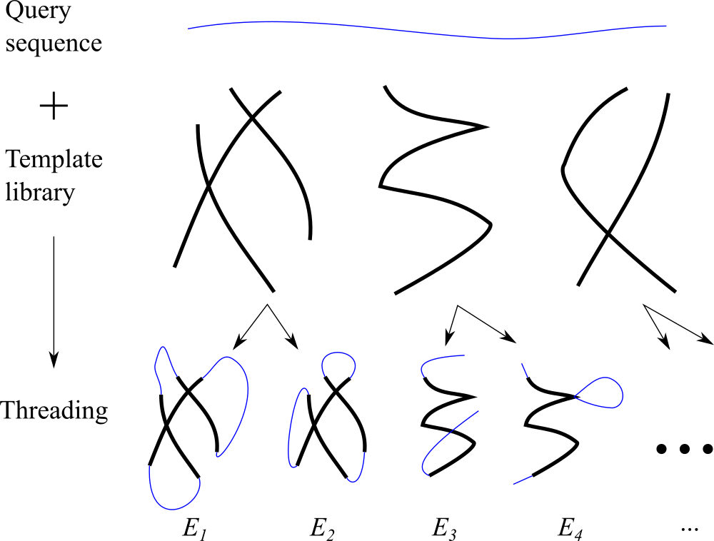
Figure 16:The basic idea of threading: a sequence is “threaded” through templates extracted from a database of known folds (e.g. the PDB), and the resulting structure is assigned an energy. The structure having the lowest energy is taken as the optimal candidate.
To recognize the fold of a chain having no visible homology with already solved proteins, one can use various superpositions of the chain in question onto all examined (taken from an a priori classification or from PDB) 3D folds in search of the lowest-energy chain-with-fold alignment, as sketched in Figure 16. This is called the threading method. When a chain is aligned with the given fold, it is threaded onto the fold’s backbone until its energy (or rather, free energy) is minimized, including both local interactions and interactions between remote chain regions. The threading alignment allows “gaps” in the chain and in the fold’s backbone (the latter are often allowed for irregular backbone regions only). Many different algorithms have been proposed for finding the correct threading of a sequence onto a structure, though many make use of dynamic programming in some form. Indeed, in principle, threading is similar to a homology search; the difference is that only sequences are aligned in a homology search, while threading aligns a “new” sequence with “old” folds.
Being physics-inspired, threading can be a powerful tool for structural biologists and biophysicists. It uses mostly statistics-derived pseudopotentials rather than actual energies, which are based on the contact statistics between amino acids as found in known protein structures[16].
As with any other structure-prediction model, there are some issues with threading, the main ones being:
The conformations of the gapped regions remain unknown, together with all interactions in these regions.
Even the conformations of the aligned regions and their interactions are known only approximately, since the alignment does not include side-chain conformations (which may differ in “new” and “old” structures). Estimates show that threading takes into account, at best, half of the interactions operating in the protein chain, while the other half remain unknown to us. Thus, again, the protein structure is to be judged from only a part of the interactions occurring in this structure. Therefore, this can only be a probabilistic judgment.
The number of possible alignments is enormous (remember Levinthal’s paradox?), which makes it very hard to sort out all possible threading alignments and single out the best one (or ones). Here there are many methods that can be employed, one of which being the statistical mechanics of one-dimensional systems, and the related dynamic programming techniques.

Figure 17:The 3D structures of (left) chicken histone H5 and (right) replication terminating protein (rtp). Note that the C-terminal helix of rtp is not shown, since it has no analoug in the histone. The root mean-squared deviation between 65 equivalent positions in the two structures is 2.4 . Taken from Flöckner et al. (1995).
As an example, Finkelstein & Ptitsyn (2016) shows the structure prediction done for the replication terminating protein (rtp) by threading. Having threaded the rtp sequence onto all PDB-stored folds, Flöckner et al. (1995) used threading with statistics-based pseudopotentials to show that the rtp fold must be similar to that of H5 histone. This a priori recognition, which is shown in Figure 17, turned out to be correct.
However, it also turned out that the alignment provided by threading deviates from the true alignment obtained from superposed 3D structures of rtp and H5 histone. On the one hand, this shows that even a rather inaccurate picture of residue-to-residue contacts can lead to an approximately correct structure prediction. On the other hand, this shows once again that all the mentioned flaws (insufficiently precise interaction potentials, uncertainty in conformations of nonaligned regions, of side chains, etc.) make it possible to single out only a more-or-less narrow set of plausible folds rather than one unique correct fold. Indeed, the set of the “most plausible” folds can be singled out quite reliably, but it still remains unclear which of these is the best. The native structure is a member of the set of the plausible ones, it is more or less close to the most plausible (predicted) fold, but this is all that one can actually say even in the very best case.
Threading methods became a tool for a tentative recognition of protein folds from their sequences. The advantage of these methods is that they formulate a recipe: do this, this and this, and you will obtain a few plausible folds, one of which has a fairly high chance of being correct.
1.5AlphaFold
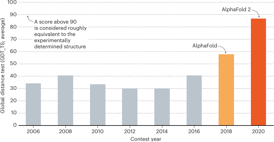
Figure 18:The performance of CASP winners in the eight contests up to 2020. Taken from Callaway (2020).
The CASP (Critical Assessment of protein Structure Prediction) contest is a biennial competition established to evaluate the performance of computational methods for protein structure prediction. Since its inception in 1994, CASP has become a benchmark for assessing progress in the field, gathering researchers from across the globe to tackle one of the most complex challenges in computational biology. Participants receive amino acid sequences of proteins for which the 3D structure remains experimentally unknown to them but has been solved by researchers outside the competition. They then attempt to predict these structures using their algorithms, which are later evaluated against the experimentally determined ones. Figure 18 shows the score of the winners of the last 8 contests. As can be seen in the figure, in 2020 there was a breakthrough that made it possible to predict the 3D structure of proteins with a precision close to the experimental one.
The breakthrough has been possible thanks to AlphaFold2 (which I will refer to simply as “AlphaFold” from now on), which is a deep learning model developed by DeepMind, presented in Jumper et al. (2021), designed to predict protein structures with remarkable accuracy. The work behind AlphaFold has been awarded half of the 2024 Nobel Prize in Chemistry. The model’s architecture is based on neural networks, and integrates several advanced techniques from machine learning and structural biology to predict the 3D structure of a protein out of its sequence (i.e., the folding problem). I will briefly describe the internal architecture of Alphafold, and then show how to use it (in a slightly improved version called ColabFold, presented in Mirdita et al. (2022)).
1.5.1Input and preprocessing
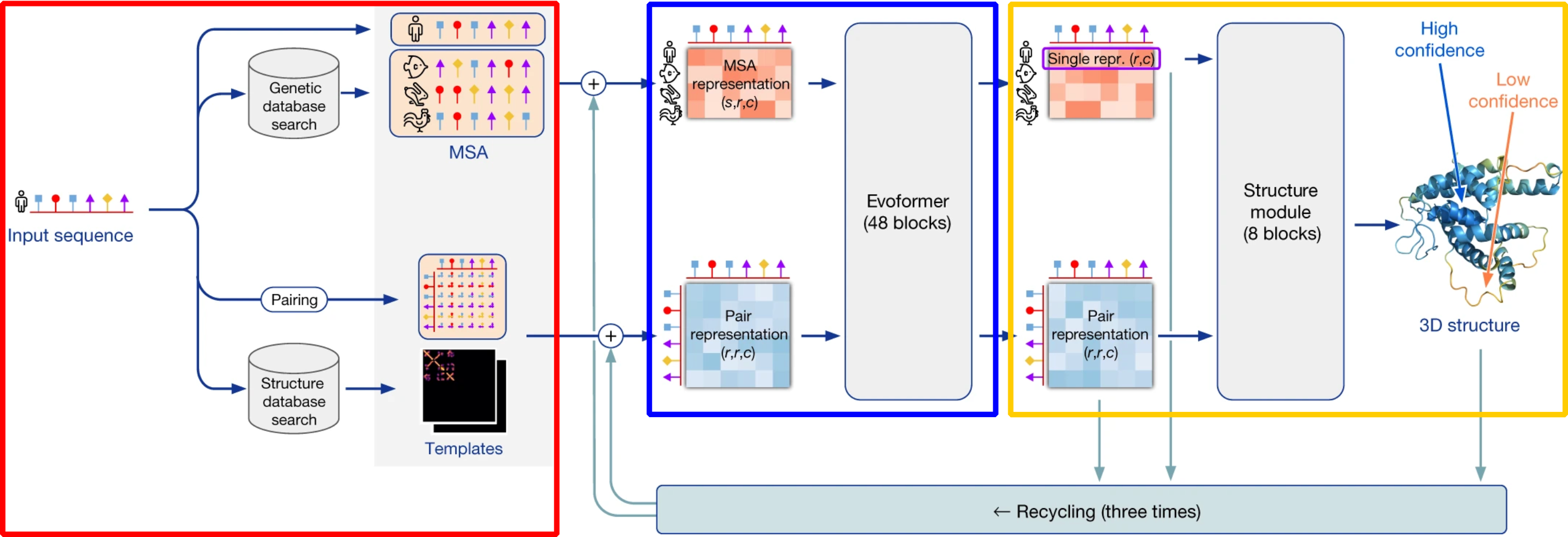
Figure 19:The architecture of AlphaFold. Arrows show how the information flows among the components. The input (preprocessing) module, the evoform and the structure module are highlighted in red, blue and yellow, respectively. Adapted from Jumper et al. (2021).
The overall architecture, as presented in the original paper, is shown in Figure 19. The first part, which handles the user input and is highlighted in red in Figure 19, is a preprocessing pipeline that can be carried out independently of the rest as done, for instance, in ColabFold. First of all, the AlphaFold system uses the input amino acid sequence to query several databases of protein sequences, and constructs a multiple sequence alignment in order to determine the parts of the sequence that are more likely to mutate. The underlying idea is that, if two amino acids (possibly far apart along the sequence) are in close spatial contact, mutations in one of them will be closely followed by mutations of the other, so that the overall 3D structure is preserved. To make an extreme (and somewhat unrealistic) example, suppose we have a protein where an amino acid with negative charge (say, glutamate) is spatially close to an amino acid with positive charge (say, lysine), although they are both far away in the sequence. Most likely, the resulting electrostatic interaction stabilises the structure of the protein. If for evolutionary reasons the first AA mutates into a positively charged amino acid, the second AA will be under evolutionary pressure to mutate into a negatively charged amino acid in order to preserve the electrostatic attraction and therefore the contribution to the stability of the folded protein. The MSA makes it possible to detect this sort of correlations.
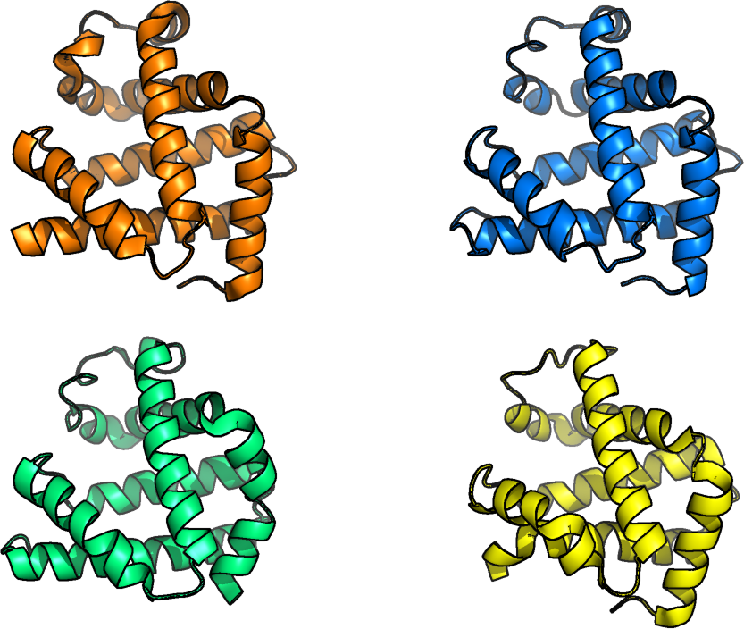
Figure 20:The 3D structure of human myoglobin (top left), african elephant myoglobin (top right, 80% sequence identity), blackfin tuna myoglobin (bottom right, 45% sequence identity) and pigeon myoglobin (bottom left, 25% sequence identity). Credits to Carlos Outeiral.
AlphaFold also tries to identify proteins that may have a similar structure to the input (“templates”), and constructs an initial representation of the structure called the “pair representation” which is, in essence, a model of which amino acids are likely to be in contact with each other. Finding templates follows a completely different, but closely related principle: proteins mutate and evolve, but their structures tend to remain similar despite the changes. In Figure 20, for example, I display the structure of four different myoglobin proteins, corresponding to different organisms. You can appreciate that they all look pretty much the same, but if you were to look at the sequences, you would find enormous differences. The protein on the bottom right, for example, only has ~25% amino acids in common with the protein on the top left.
1.5.2The Evoformer
For years, the use of MSAs to detect correlations between amino acids relied on statistical analysis, but its limited accuracy required substantial improvements. Early breakthroughs in coevolutionary analysis helped identify biases in the data and correct them using more advanced statistical techniques. These methods contributed to better but still imperfect predictions of protein structures.
In AlphaFold, the information about the MSA and the templates is jointly analysed by a special type of transformer, which is a deep learning method introduced in Vaswani et al. (2017) that uses a mechanism called attention, allowing the model to focus on different parts of the input data, assigning varying importance to specific regions. This architecture became popular in tasks like natural language processing (NLP) due to its ability to model long-range dependencies in sequences. Instead of processing data sequentially, transformers look at all parts of the input simultaneously, which significantly speeds up learning and makes it more efficient. In bioinformatics, this approach has been adapted to analyze MSAs, improving how relationships between residues are understood. AlphaFold takes the application of transformers a step further with its Evoformer architecture (highlighted in blue in Figure 19), which processes both the MSA and the templates, allowing information to flow back and forth between the sequence and the structural representations. Unlike previous deep learning approaches, where geometric proximity was inferred only at the end, AlphaFold continuously updates and refines its structural predictions throughout the process.
Evoformer uses a two-tower transformer model, with one tower dedicated to the MSA (called the MSA transformer) and the other focusing on pairwise residue interactions (pair representation). At each iteration, these representations exchange information, improving both the understanding of the sequence and the predicted pair representation. This iterative refinement, performed 48 times in the published model, allows AlphaFold to adjust its predictions based on both the sequence data and evolving structural hypotheses.
For example, if the MSA transformer identifies a correlation between two residues, it hypothesizes that they are spatially close. This information is passed to the pair representation, which updates the structural model. The pair transformer can then detect further correlations between other residues, perhaps close to the first pair, refining the structure hypothesis. This back-and-forth exchange continues until the model reaches a confident structural prediction.
Note that this step is particularly memory intensive, since the construction of the attention matrix in trasformers has a quadratic memory cost, which can bring down to their knees even powerful GPUs, making it hard to use AlphaFold to predict the structure or long proteins on consumer hardware.
1.5.3The structure module
The information generated by the Evoformer is taken to the structure module (highlighted in yellow in Figure 19). The idea behind the structure module is conceptually very simple, but its implementation is fairly complex.
The structure module considers the protein as a “residue gas”: every AA is modelled as a triangle, representing the three atoms of the backbone. These triangles float around in space, and are moved by the network to form the structure. The transformations are parametrised as 4x4 affine matrices that handle rotations and translations. At the beginning of the structure module, all of the residues are placed at the origin of coordinates. At every step of the iterative process, AlphaFold produces a set of affine matrices that displace and rotate the residues in space. This representation does not reflect any physical or geometrical assumptions, and as a result the network has a tendency to generate structural violations. This is particularly visible in the supplementary videos of Jumper et al. (2021), that display some deeply unphysical snapshots (see Figure 21 for a striking example).
Figure 21:The evolving prediction of the CASP14 multi-domain target (863 residues) T1091. Individual domains’ structure is determined early, while the domain packing evolves throughout the network. The network explores unphysical configurations throughout the process, resulting in the long “strings” that appear during the evolution. Supplementary Video 4 of Jumper et al. (2021), which can be downloaded here.
The secret sauce of the structure module is a new flavour of attention devised specifically for working with three-dimensional structures which is based on the very simple fact that the L2-norm of a vector is invariant with respect to translations and rotations[17]. Why is this invariance such a big deal? You may understand this as a form of data augmentation: if the model knows that any possible rotation of translation of the data will lead to the same answer, it will need a lot less data to pull it away from wrong models and will therefore be able to learn much more.
Finally, it is also worth noting that the Structure Module also generates a model of the side chains. To simplify the system, their positions are parametrised by a list of dihedral angles , , etc. (depending on the AA), which are predicted in their normal form by the network, and implemented with standard geometric subroutines.
1.5.4Recycling and loss function
AlphaFold leverages a so-called “recycling mechanism”: after generating a final structure, it takes all the information (i.e. the MSA and pair representations, as well as the predicted structure) and passes it back to the beginning of the Evoformer blocks. In the original paper the whole pipeline is executed three times.
The quality of the training and of the final output of AlphaFold are determined by a specialized loss function called Frame Aligned Point Error (FAPE), a modified version of RMSD, to align atomic positions, which helps prevent incorrect protein chirality. However, this is only part of a more complex loss function, which is a weighted sum of various auxiliary losses. These include losses calculated from multiple iterations of the structure module and a distogram loss, which compares predicted 2D distance matrices with the true structure.
Another interesting aspect is MSA masking, inspired by self-supervised learning models, where some symbols in the MSA are masked and the model is asked to predict them. An additional trick employed is the so-called self-distillation: in this approach, they took a model trained exclusively on the PDB, and predicted the structures of ~300k diverse protein sequences. They then retrained the full model, incorporating a small random sample of these structures at every training cycle. The claim is that this operation allows the model to leverage the large amount of unlabelled data available in protein sequence repositories.
1.5.5Output
The single most useful output of AlphaFold is the 3D coordinates of each atom of the final predicted structure. A very important metric that is reported by the model is the predicted local-distance difference test (pLDDT), which provides a per-residue confidence score on a scale from 0 to 100, indicating how certain the model is about the position of each amino acid in the predicted 3D structure. A higher pLDDT score suggests greater accuracy, with scores above 90 being highly reliable, while scores below 70 indicate regions with lower confidence, possibly due to disorder or flexibility. Finally, AlphaFold also outputs a distogram, which is a histogram of pairwise distances.
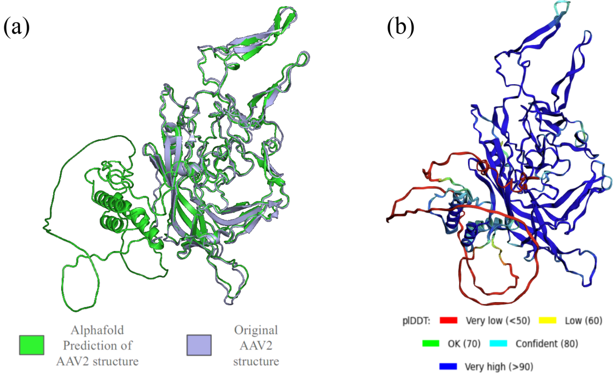
Figure 22:(a) The superposition between the experimental and Alphafold-predicted structures of the VP1 protein composing the capsid of a AAV2 virus. (b) The Alphafold-predicted structure, coloured according to the value of the pLDDT of each residue. Courtesy of Mouna Ouattara.
Figure 22 shows an example where Alphafold was used to predict the structure of a protein that makes up part of a viral capsid. Since the experimental structure is available, it is possible to superpose it to the predicted structure, which shows that a part of the latter has been hallucinated, i.e. made up, by Alphafold. Interestingly, a large part of the hallucinated portion is predicted to be a coil and has a very low pLDDT, but part of it (the two helices) is structured and has a good pLDDT.
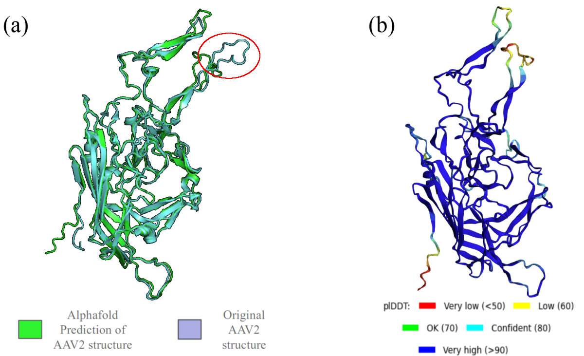
Figure 23:Same as Figure 22, but for a mutant serotype (7m8, see Dalkara et al. (2013)), which differs from the wildtype for a 10-amino acid peptide insertion in the VR-VIII loop, highlighted with a red ellipse in panel (a). Courtesy of Mouna Ouattara.
By contrast, Figure 23 shows the same comparisons for a closely related protein, which is obtained by adding a short peptide (10 amino acid long) to a loop that is far apart from the part of the protein that Alphafold hallucinates when predicting the structure of the wildtype protein. Nevertheless, in this case the predicted structure is very close to the experimental one.
1.5.6Using AlphaFold through ColabFold
ColabFold, presented in Mirdita et al. (2022), is an optimized implementation of AlphaFold that runs on Google Colab, providing a more accessible and user-friendly way to perform protein structure predictions. Unlike the “pure” AlphaFold, which can be downloaded here and requires extensive computational resources and a setup that may be challenging for individual users, ColabFold makes AlphaFold’s capabilities more widely available by leveraging Google’s cloud infrastructure. The ColabFold version is streamlined for easier use and has a faster input preprocessing, with the option to use precomputed databases for sequence searching, that significantly reduces both runtime and storage requirements. ColabFold provides an easy way to customise the most common options of the model, allowing users to adjust parameters, access multi-sequence alignments, and use additional input sequences to improve prediction accuracy. The code behind the notebook is open source (see here), and the notebook itself can be accessed here.
2Nucleic acids
As for proteins, the structure of nucleic acids can be studied at different levels. The primary structure is the unidimensional list of nucleotides, which can be obtained fairly easily through sequencing. In DNA and RNA, the secondary structure is the list of base pairs that are formed between different parts of the strand(s), while the 3D structure is the description of how the polymer bends and twists. Here, contrary, to proteins, attractive interactions beyond base pairing (which includes stacking) are not very strong, and since nucleic acids are hydrophilic, there is no strong tendency of the nucleotides to tightly pack together. As a result, the free energy that stabilises a molecule’s conformation mostly comes from the secondary (rather than tertiary, as in proteins) structure. Therefore, there are many useful things that we can learn about a certain RNA or DNA system by just knowing its secondary structure.
Here I will present methods and algorithms that have been developed for single chains of RNA, but they are mostly valid for (or extendable to) multi-stranded and DNA systems. Formally, given a chain of length , a secondary structure can be represented as a graph where each nucleotide is a vertex, and each base pair is an edge connecting two vertices. The connectivity can be represented by an adjancency matrix , where each element of the matrix is equal to 1 if and are linked (either through the backbone or by hydrogen bonds) and 0 otherwise. In the case of the single chain, nucleotides are ordered and the backbone is continuous, thus . Moreover, since each nucleotide can be involved in most one base pair, for each there is at most one different from and for which .
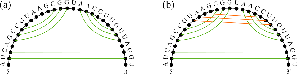
Figure 24:Possible secondary structures of an RNA strand of sequence AUCAGCCGUAAGCGGUAACCUUGUUAGGU, represented as graphs. The points are the nucleotides (i.e. the graph’s vertices), while lines that connect them are the graph’s edges. The black and coloured lines are the exterior and interior edges, respectively. In (a) no lines cross, while in (b) there are intersections between orange and green lines: a pseudoknot is present.
Note that secondary structure prediction becomes much easier if we assume that no pseudoknots can form. This is a strong assumption, but it is very convenient from an algorithmic point of view. In the graph/matrix representation, this condition is fulfilled if, for any pair of base pairs and ,
if then ;
if then .
In the graph representation, pseudoknots are present if some edges intersect. Figure 24 shows the secondary structure (with and without knots) of a short RNA strand, represented as a graph.
Now we want to predict the secondary structure of the RNA, given its sequence. Since here we are dealing with one-dimensional sequences, I hope it will not be surprising to know that dynamic programming can be leveraged to find a solution to this problem, provided that
we use a scoring scheme whereby the free-energy contribution that each base pair (or, more generally, “local” secondary structure motif) has on the overall stability of the molecule is additive;
we assume that pseudoknots cannot form, so that the RNA can be split into two smaller ones which are independent.
Indeed, under these conditions the solution to the full problem can be built by solving subproblems, which can be done efficiently by applying dynamic programming. The next two sections will describe two algorithms that can be used to obtain the optimal structure, i.e. the one with the minimum free-energy (MFE).
2.1Nussinov’s algorithm
The first approach I will describe has been introduced by Nussinov et al. (1978). To keep it simple, I will use a version of the algorithm in which the (free) energy of an unpaired base is 0, and that of a base pair is a fixed value, i.e. -1, regardless of the type of nucleotides involved.

Figure 25:The graph representation of Nussinov’s recursive relation. Given a subsequence , is either unpaired (first term after the equal sign), or is paired to some other nucleotide .
The intuition behind Nussinov’s algorithm, shown pictorially in Figure 25, is the following: for any subsequence , , the -th base can either remain unpaired or be paired with some -th base where . If the -th base is unpaired, the (free) energy of , denoted as , simply reduces to the energy of the subsequence , or . This forms the first term of the Nussinov recurrence relation.
On the other hand, if the -th base pairs with the -th base, then consists of the energy contribution of this pairing, denoted as , plus the energies of the two resulting subproblems: the subsequence , represented by , and the subsequence , represented by . Finding the optimal that minimizes this value gives us the second term in the Nussinov recurrence relation.
Therefore, the optimal energy of the subsequence is the minimum of the energy when the -th base is unpaired and the energy when it is paired with the optimal -th base, which can be written explicitly as follows:
In this case the dynamic programming table is of size , and is initialised so that its diagonal entries are set to zero, since a nucleotide cannot bind to itself. The other entries are set iteratively by starting from the bottom-right entry, where and , so that the matrix is progressively filled up from left to right and bottom to top. The final score, representing the optimal solution for the entire sequence, is found in the upper right corner of the matrix, corresponding to the subsequence . Since each entry requires an minimisation, and there are entries, the total algorithmic complexity is .
As always with dynamic programming methods, the secondary structure is obtained by using a traceback matrix , which is initialised during the fill-in phase. In particular, given the optimal secondary structure of the subsequence , if is unpaired, while , where is the nucleotide that is paired to , otherwise. A possible recursive traceback function is
DEFINE K as the traceback matrix K
DEFINE P as the list of base pairs

FUNCTION traceback(i, j)
    k = K(i, j)
    IF i > j
        RETURN
    IF k == 0
        traceback(i + 1, j)
    ELSE
        ADD (i, k) TO P
        traceback(i + 1, k - 1)
        traceback(k + 1, j)
The recursion starts from the end, i.e. with i = 0 and j = N - 1, and at the end of the procedure the list of base pairs is stored in P.
Note that the complexity of the traceback algorithm is , since we move through a matrix and perform a operation on each entry we visit.
The Nussinov’s algorithm is quite simplistic and comes with several limitations. In its naive implementation, the algorithm does not account for some important factors in RNA folding. Most notably, it does not take into account that, as we already know, stacking interactions between neighboring base pairs are crucial for RNA stability, at least as much as hydrogen bonding. To address this and other limitations, it is fundamental to incorporate biophysical factors into the prediction model. One improvement is to assign energies to structural elements rather than to individual base pairs, so that the total energy of the RNA structure becomes the sum of the energies of these substructures.
2.2Zuker’s algorithm
Most of the issues mentioned above can be overcome with the algorithm devised by Zuker and Stiegler. The algorithm is based on the idea that RNA folds into a structure that minimizes its free energy, taking into account not only base pairing, but also other factors. In particular, the algorithm assumes that the RNA folding process can be described by an energy model where base pairs, stacking interactions, and loops (hairpin loops, bulge loops, interior loops, and multi-branch loops) contribute to the total free energy of the molecule. The Turner energy model is commonly used in implementations, which provides empirical parameters for these contributions.

Figure 26:Two schematic representations of the secondary structure of a simple RNA molecule. (a) The conventional representation. (b) The same structure, represented as an undirected graph with exterior and interior edges. The legend in the bottom right applies to both panels. Note that here “bifurcation loop” is used in place of multibranched loop. Taken from Zuker & Stiegler (1981).
The key idea can be fully appreciated by representing an RNA secondary structure as an undirected graph, drawn as a semicircle with chords connecting some edges (see also Figure 24). In the following description I borrow heavily from the original paper, which still is (after more than 40 years) one of the best resources on the subject[19]. Here are a few definitions:
the nucleotides are the vertices of the graph;
the arcs that connect each pair of and nucleotides are the exterior edges and represent the backbone bonds;
chords connecting vertices represent base pairs, and therefore connect only complementary nucleotides (C-G, A-U or G-U); these chords are called interior edges and have the following properties:
interior edges do not touch, since each nucleotide can be involved in no more than one base pair;
interior edges do not cross, since pseudoknots are not allowed.
a face is a region of the graph that is bounded on all sides by edges.
These definitions are pictorially represented in Figure 26. The difference with Nussinov’s algorithm is that the (free) energy of a structure is associated not with the base pairs, but with the regions that are bounded by the bonds, i.e. with the graph faces associated to that structure. Indeed, the possible secondary structure motifs can be classified according to how they can be represented in terms of faces:
A face bounded by a single interior edge is a hairpin loop, whose length is the number of exterior edges (the number of nucleotides composing the loop is this number minus one);
A face bounded by two interior edges is further classified into three groups:
if the interior edges are separated by two single exterior edges on both sides, the face is a stacking region (or stacking loop);
if the face is bounded by a single exterior edge on one side, and multiple exterior edges on the other, the face is a bulge loop;
if there are multiple exterior edges on both sides, the face is an interior loop;
A face that has () interior edges is a -multiloop (or a multibranched loop of order ).
The energy of a given structure is the sum of the energies associated to each of its faces, . This is a powerful way of setting the statistical weight of each motif by using experimentally-determined values: for instance, since hairpins with loops shorter than 3 are not possible, we can assign the energy to hairpin loops having fewer than four exterior edges. Any other specific effect (e.g. complicated sequence-dependent effect) can be naturally incorporated in this framework.
Thanks to this decomposition, if we know (or can estimate) the energy contributions associated to each secondary structure motif, we can compute the total energy of any given structure. However, enumerating all possible structures to find the one with the lowest (free) energy would be computationally impossible even for rather small sequences. The problem can be overcome by using dynamic programming, with an approach similar (but not equal) to that of Nussinov.
As before, is the subsequence . For each we define
as the minimum free energy of the subsequence;
as the minimum free energy of all structures formed by , in which and are paired with each other; if and cannot pair with each other, .
The constraint on the minimum length of hairpin loops can be enforced by setting if , while is initially set to 0. By constrast, if , and can be written in terms of and for various pairs for which , i.e. in terms of the minimum energies of smaller substructures. The recursive relations for the two matrices, and , both of size , can be found by considering the possible structures formed by .

Figure 27:Possible substructures for the subsequence , constrained to the presence of an edge. Adapted from Zuker & Stiegler (1981).
We start with . First of all, note that this matrix considers only those substructures that have and paired or, in other words, substructures whose graph representation has the interior edge. The presence of this additional edge means that the resulting optimal substructure also has an additional face compared to any other substructure that has been already evaluated. In particular, as shown in Figure 27,
can close a hairpin, thus contributing with an energy ;
can close a face containing exactly two interior edges, with the other edge being , with . The face contributes an energy that depends on the face which, as before, can be of three types:
and : the face is a stacking region;
or (but not both): the face is a bulge region;
and : the face is an interior loop.
can close a face containing interior edges, with the other edges being . This is a -multiloop, and its energy contribution is .
In all these cases, the , and penalty functions are model parameters, and can be estimated by experiment (see the section on nearest-neighbour models). Of course, there are multiple substructures in which the edge is present. We make sure to select the one with the lowest free energy by first obtaining the single optimal substructures that fall into cases 2. and 3., and then by picking the optimal substructure among the three possibilities listed above. This procedure translates to the following recursive relation:
where is the energy associated to the possibility that the new face is a stacking region, for which we do not have to carry out any minimisation, since we already know that and .

Figure 28:Possible substructures for the subsequence , this time with no constraints. Adapted from Zuker & Stiegler (1981).
Now we can write down the recursive relation for . There are once again three possibilities, shown schematically in Figure 28:
and (one of them or both) do not form base pairs in the substructure. Since dangling ends do not contribute to the overall energy, or .
and form a base pair. In this case , which we have already computed.
and base pair, but not with each other. In other words, there exist interior edges and (with ). In this case there is an “open bifurcation”, as the energy can be written in terms of two substructures: .
The last case requires a minimisation over (or, equivalently ), which translates to the following recursive relation:
The recursive relations for and can be used in a dynamic programming code to obtain the optimal secondary structure of the full sequence . Since there is the constraint on the minimal loop length, after initialisation we start filling the matrices from the entry, and continue from bottom to top and from left to right. As in Nussinov’s algorithm, the energy of the optimal structure of the entire sequence will be stored at the end of the fill-in phase in the entry, and the optimal secondary structure itself can be retrieved by using traceback matrices.
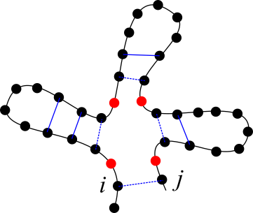
Figure 29:An example of a multibranched loop with and . Interior edges are coloured in blue, while the interior edges that define the multiloop are drawn with dashed lines. Unpaired nucleotides within the loop are coloured in red.
What is the algorithmic complexity of the method? In the last case of Eq. (48), we minimise on the order of the multiloop, and on all its interior edges. This operation has an exponential complexity, and therefore completely kills the computational efficiency. There exist several approximations that can be leveraged to obtain a polynomial complexity. The most extreme one is given by Eq. (50), which completely neglects the energetic penalty of the multiloop. A more realistic approximation is the following:
where is the order of the loop, is the number of unpaired bases within the loop (see Figure 29), and , and are parameters, to be estimated experimentally. This approach makes use of another auxiliary matrix, , whose generic entry is the optimal energy of , with the constraint that and are part of an open multiloop. Since there is no valid “empty” multiloop state, initially all entries are set to zero, i.e. . The recursive relation takes into account the possibilities that and/or are unpaired, which contributes , or are paired with each other, which contributes , and therefore
We can now rewrite the last case of Eq. (48) by making use of the new matrix, obtaining
where the latter contribution takes into account the presence of a multiloop closed by and . Note that the same result can be obtained more cleanly by using another auxiliary matrix, which makes integration with additional terms (*e.g. dangling ends) a bit more straightforward. The algorithmic complexity of the four cases are , , and . Since there are entries, the overall algorithmic complexity is , and the required storage space is , since only matrices are used. The computational efficiency can be improved by limiting the size of a bulge or interior loop to some value (often taken to be 30), which brings the complexity of the third case of Eq. (56) down to , and the overall algorithmic complexity down to .
A very nice (but not necessarily easy to read) open-source implementation of the Zuker’s algorithm can be found here.
2.3Beyond the MFE: the McCaskill algorithm[20]
The Nussinov’s and Zuker’s algorithm find the optimal secondary structure of an RNA strand, defined as the structure that minimise the overall (free) energy. However, the conformations of macromolecules that are in thermal equilibrium with their environment are not fixed: in principle any allowed structure can be visited, given enough time (remember the concept of ergodicity and phase space?). In particular, if we define as the structural ensemble, i.e. the ensemble of allowed structures, the probability that a macromolecule has a specific secondary structure is given by
where is the energy of secondary structure , and is the partition function. We now look for a recursive relation to compute the partition function of a sequence . Given a subsequence , is either unpaired, or it is paired with the -th nucleotide, where . For the first case, the partition function is that of the smaller subsequence , . For the latter case, the edge splits the subsequence in two independent subproblems, and the overall partition function is given by the product of their partition functions, and , where is the statistical weight of the base pair formed by and . Look at Figure 25 and you will realise that it is the same splitting! The total partition function will be a sum over all these cases, viz
This relation makes it possible to write down a dynamic programming code that fill the matrix with a complexity . As before, the partition function of the sequence is found in the entry.
How can we use the information contained in the partition function to obtain the equilibrium (structural) ensemble of the strand? The most granular information we can compute is the probability that two nucleotides and are base paired, . However, in order to do so we first have to introduce the auxiliary matrix , whose generic entry stores the partition function of the subsequence , with the constraint that nucleotides and form the base pair. Its recursive relation is
so that the recursive relation of (Eq. (58)) becomes
Note that with this formalism it is easier to employ more realistic energy functions by adding contributions (due to interior and multiloops, for instance) to Eq. (59), in analogy with the strategy devised by Zuker. See here for additional details.

Figure 30:A graph where the base pair is (a) external and (b) enclosed by an base pair.
We can write down the probability recursively, as the sum of two contributions, shown graphically in Figure 30:
The probability that the edge exists and it is external, i.e. that there are no edges for which . In this case the base pair split the graph into three independent parts, so that the total probability is just
The probability that the edge exists and it is enclosed by other base pairs. This is a sum over all the possible enclosing base pairs , with , of the probability that the edge exists, , times the probability that the edge is the exterior edge of the subsequence, which is given by[21]
All in all, this contribution amounts to
The total probability that and form a base pair is thus
Note that the algorithmic complexity of this computation is , since there is the double sum over and , which has to be carried out for every pair. However, the complexity can be brought down to by introducing another auxiliary matrix (see e.g. Bernhart et al. (2011)).
2.4Third-party software
You can find several codes online implementing the algorithms we just discussed. However, many of them are a bit rough around the edges and/or incomplete (or wrong). Some interesting and well-done open source implementations are available in different languages. seqfold implements the Zuker algorithm for both DNA and RNA, and it is a rather readable code written in Python. At this website there are several pages where you can test “RNA algorithms” (several of which we already introduced). Interestingly, the authors (from Freiburg University) also released an excellent paper detailing their implementations, as well as their code.
The current state-of-the-art software codes for RNA folding are RNAfold, bundled in the ViennaRNA package, and mFold, which was originally developed by M. Zuker and is been since merged with other packages in the UNAFold software. Both softwares can be used online as webservers, but can also downloaded and installed locally. However, ViennaRNA can be downloaded freely, while UNAFold requires a license (although older versions of mFold can be freely downloaded here).
The best online webserver is surely the one based on ViennaRNA, which can be found here. It provides tools to do almost everything related to RNA secondary structures, and I invite you to use it (and possibly read the accompanying papers). The tool that implements the algorithms of Zuker and McCaskill is RNAfold. Try it, and compare its predictions to those of the simple codes we discussed in class.
2.4.1NUPACK
An online webserver, which is also a Python library, that has a slightly different scope but uses algorithms that are very much inline with those we just studied, is NUPACK. The most recent NUPACK version is described here. NUPACK has been free-to-use for many years, but it is apparently on the verge of requiring a paid subscription to use its webservices. By contrast, for now the Python library, which has an open-source-like license for non-commercial academic use, is free-to-download here, provided that you are a registered user.
I want to briefly describe what NUPACK does, and why it is one of the most used software by the DNA/RNA nanotechnology community. At its core, NUPACK integrates statistical thermodynamics and advanced algorithms to model the folding, hybridization, and thermodynamic stability of nucleic acids. The main appeal of NUPACK compared to other packages lies in its ability to model multi-strand nucleic acid systems. In contrast to simpler single-strand predictions, many DNA nanotechnology applications involve multiple strands interacting to form complex assemblies. NUPACK handles these multi-stranded configurations by extending the core ideas found in the classical algorithms we studied, generalizing them to more complicated systems where the combinatorial possibilities of base-pairing grow exponentially not only with the number of nucleotides, but also with the number of strands.
In practical terms, NUPACK enables researchers to predict the secondary structures that DNA or RNA strands will adopt under given conditions. NUPACK’s algorithms minimize free energy to predict the most stable structure, but also consider an ensemble of possible structures, going beyond the minimum free energy configuration. Indeed, it uses McCaskill-like algorithms to compute the partition function, providing information about the entire landscape of possible configurations. Going beyond folding, NUPACK can also design sequences for specific structures: In nanotechnology, designing DNA or RNA that reliably folds into a desired structure is essential for creating functional nanodevices or molecular machines. NUPACK optimizes nucleotide sequences to favor specific target structures while minimizing the formation of undesired alternatives, often through iterative sequence design techniques rooted in statistical optimization.
In another context, that of first-order phase transition, we would say “once a nucleus forms”.
Note that in the original Zimm-Bragg model the first three segments are always in the coil state, so that the exponent is rather than .
There is a typo in the Appendix B of Finkelstein & Ptitsyn (2016): the element of should be -1 and not 1.
For the chain lengths usually considered, the ratio of the numbers of residues exposed to the solvent or buried in the protein core is closer to that of real proteins compared to 3D lattices (see Moreno‐Hernández & Levitt (2012) and references therein).
Which values are “too large” depend on the hardware and algorithms used to write the code.
Here I’m abusing the notation by using the same symbol to represent two different (but very related) quantities.
Note that this is not the only possible choice: we could choose a probabilistic method, for example using Hidden Markov Models (HMMs), that would assign a probability measure over the space of possible event paths and use other methods for evaluating alignments (e.g., Bayesian methods).
Horizontal gene transfer is the movement of genetic material between organisms in a manner other than traditional reproduction (vertical inheritance). This process allows genes to be transferred across different species, leading to genetic diversity and the rapid acquisition of new traits, and can occur through several mechanisms.
Indels (shorthand for “insertions/deletions”) that cause frame-shifts in functional elements generally cause important phenotypic modifications.
It is also valuable in cases where one sequence may be a subsequence of another, like when searching for a gene within a cromosome or a whole genome.
It is clear that in this context and are part of larger sequences.
For DNA words, common parameters are +5/-4 or +2/-3 for matches and mismatches.
It is possible to derive expressions that use effective rather than true sequence lengths, to compensate for edge effects (an alignment that starts near the end of the query or database sequence is likely not to have enough sequence to build an optimal alignment).
There are many!
Similar, in spirit, to the way substitution matrices are computed.
An explanation of this Invariant Point Attention (IPA) is well-beyond my expertise. If you are interested, I refer to section 1.8 of the Supplementary Information of the original paper.
This ATPase is a homodimer.
It is very common for papers that contributed greatly to a field to be also very well thought out and written. This is only partially true for the paper in question (as mentioned below).
The derivations in this section are taken from Raden et al. (2018).
Eq. (10) of Raden et al. (2018) is written slightly differently, since they use the fact that
- Finkelstein, A. V., & Ptitsyn, O. (2002). Protein physics: a course of lectures. Elsevier.
- Bialek, W. (2012). Biophysics: searching for principles. Princeton University Press.
- Zhou, Y., Hall, C. K., & Karplus, M. (1999). The calorimetric criterion for a two‐state process revisited. Protein Science, 8(5), 1064–1074. 10.1110/ps.8.5.1064
- Anfinsen, C. B., Haber, E., Sela, M., & White, F. H. (1961). THE KINETICS OF FORMATION OF NATIVE RIBONUCLEASE DURING OXIDATION OF THE REDUCED POLYPEPTIDE CHAIN. Proceedings of the National Academy of Sciences, 47(9), 1309–1314. 10.1073/pnas.47.9.1309
- Anfinsen, C. B. (1973). Principles that Govern the Folding of Protein Chains. Science, 181(4096), 223–230. 10.1126/science.181.4096.223
- Onuchic, J. N., Wolynes, P. G., Luthey-Schulten, Z., & Socci, N. D. (1995). Toward an outline of the topography of a realistic protein-folding funnel. Proceedings of the National Academy of Sciences, 92(8), 3626–3630. 10.1073/pnas.92.8.3626
- Zimm, B. H., & Bragg, J. K. (1959). Theory of the Phase Transition between Helix and Random Coil in Polypeptide Chains. The Journal of Chemical Physics, 31(2), 526–535. 10.1063/1.1730390
- Doty, P., & Yang, J. T. (1956). POLYPEPTIDES. VII. POLY-γ-BENZYL-L-GLUTAMATE: THE HELIX-COIL TRANSITION IN SOLUTION1. Journal of the American Chemical Society, 78(2), 498–500. 10.1021/ja01583a070
- Badasyan, A., Giacometti, A., Podgornik, R., Mamasakhlisov, Y., & Morozov, V. (2013). Helix-coil transition in terms of Potts-like spins. The European Physical Journal E, 36(5). 10.1140/epje/i2013-13046-7
- Finkelstein, A. V., & Ptitsyn, O. (2016). Protein physics: a course of lectures. Elsevier.
- Badasyan, A. V., Giacometti, A., Mamasakhlisov, Y. Sh., Morozov, V. F., & Benight, A. S. (2010). Microscopic formulation of the Zimm-Bragg model for the helix-coil transition. Physical Review E, 81(2). 10.1103/physreve.81.021921
- Chan, H. S., & Dill, K. A. (1989). Compact polymers. Macromolecules, 22(12), 4559–4573. 10.1021/ma00202a031
- Dill, K. A. (1990). Dominant forces in protein folding. Biochemistry, 29(31), 7133–7155. 10.1021/bi00483a001
- Lau, K. F., & Dill, K. A. (1989). A lattice statistical mechanics model of the conformational and sequence spaces of proteins. Macromolecules, 22(10), 3986–3997. 10.1021/ma00200a030
- Moreno‐Hernández, S., & Levitt, M. (2012). Comparative modeling and protein‐like features of hydrophobic–polar models on a two‐dimensional lattice. Proteins: Structure, Function, and Bioinformatics, 80(6), 1683–1693. 10.1002/prot.24067