Quantum mechanics provides a rigorous framework for describing the behavior of molecules that explicitly includes the effect of the electrons. However, the calculations are very heavy and thus the evolution of a system can be followed for short times only. In addition, the computational complexity of simulating quantum systems often scales super-linearly with the size of the problem[1]. This poses significant challenges when attempting to model large-scale many-body systems accurately and for long times.
One of the fundamental distinctions between quantum and classical approaches lies in the treatment of electron contributions. In quantum calculations, the interactions and motions of electrons are computed explicitly, for instance with DFT methods, as discussed in the previous Chapter. This level of detail enables precise predictions of electronic structure and properties but comes at a high computational cost, particularly as the number of electrons and/or atoms increases.
In contrast, classical force fields adopt a simplified approach where the contributions of electrons are averaged out. Instead of explicitly modeling individual electron behaviors, classical force fields approximate the interactions between atoms using simplified mathematical models based on classical mechanics. Note that there exist also “mixed” methods, where some degrees of freedom are accounted for by using a quantum-mechanical treatment, while others are treated classically, e.g. the nuclear degrees of freedom in the CPMD approach.
In the rest of the Chapter (unless stated otherwise), we consider systems composed of interacting point particles following Newton’s equations of motion set by a classical Hamiltonian:
where and are the momentum and coordinates of particle , is its mass and is the total potential energy.
1Molecular dynamics
In a molecular dynamics simulation, the atoms, or particles, follow Newton’s equations of motions. As a result, the dynamics happens on a hypersurface defined by , where is the energy of the system. In practice, the equations of motions are solved iteratively by discretising time: the quantities of interest (position , velocity and force ) at time are used to obtain those at time , where is the integration time step. The flow of a simple MD program is:
The simulation parameters (e.g. temperature, density, time step) are read and initialised.
The initial configuration (i.e. the initial positions and velocities) is read or generated.
The simulation runs, iterating the following steps:
The forces (and possibly torques) on all particles are computed.
The positions and velocities are updated according to Newton’s equations.
The simulation stops when some condition is met (e.g. number of steps run).
The following snippet shows a pseudo-code implementation of the foregoing algorithm:
CALL initialise_parameters()
CALL initialise_system()

WHILE t is smaller than t_max
   CALL compute_force()
   CALL integrate()
   t += delta_t
   CALL sample_observables()
Program 1:Pseudo-code for a simple molecular dynamics code.
1.1Initialisation
Initialising a simulation is a trivial task when simulating simple systems, e.g. gases, most liquids and even many solids, but can become extremely difficult for highly heterogeneous systems interacting through complicated, and possibly steep, interactions. Biomacromolecules modelled at the all-atom level are definitely within this class of systems.
In general, the initial configuration should be such that there is no sensible overlap between the system’s constituents (atoms, molecules, particles, etc.), in order to avoid large initial forces that could lead to numerical instabilities that could lead to crashes or, which is worse, unphysical behaviour, such as two chains crossing each other. For simple systems this can be done in several ways:
Particle coordinates are chosen randomly one after the other, ensuring that the distance between the new particle and any other particle is larger than a given threhsold. This works great as long as the density is not too high.
Particles are placed on a lattice, making it possible to generate highly dense systems.
For more complicated systems, the generation of the initial configuration is often done in steps. In some cases, and I will show some examples, it is also common to run short-ish simulations where the dynamics is constrained (e.g. some degrees of freedom such as bond lengths or angles are kept fixed) and the energy is minimised to remove (part of) the initial stress.
In the case of highly heterogeneous systems, it is very common to use external tools to build part of (or the whole) system. Take for instance the simulation of protein-membrane systems (e.g. Figure 21), where one has to build a membrane with a given composition and density, embed one or more proteins, add ions and solvate the system.
What about velocities (or, in general, momenta)? Here initialisation is more straightforward, but there are some subtleties that can lead to errors later on if one is not careful. First of all, recall that, in a system in thermal equilibrium,
where is the -th component of the velocity of particle . We can then define the instantaneous temperature of a system of particles[2] as
where is the dimensionality of the system. We now use this relation in the following initialisation procedure:
Randomly extract each velocity component of each particle from a distribution with zero mean. A good choice is a Gaussian, but a uniform distribution will also do (but don’t be lazy!).
Set the total momentum of the system to zero by computing and subtracting it from each .
Rescale all velocities so that the initial temperature matches the desired value , i.e. multiply each component by .
If you chose to use a Gaussian distribution for step 1., then you will end up with velocities distributed according to the Maxwell-Boltzmann probability distribution at temperature , viz.
However, since the initial configuration is most likely not an equilibrium configuration, the subsequent equilibration will change the average temperature, so that . We will see later on how to couple the system to a thermostat to enforce thermal equilibrium at the desired temperature.
1.2Reduced units
In molecular simulations, reduced units are employed to simplify calculations by scaling physical quantities relative to characteristic properties of the system, such as particle size or interaction strength. This approach not only makes the equations dimensionless and more general, but it also prevents the numerical instability that can arise from dealing with values that are extremely small or large, which can occur when using standard physical units (e.g. SI units). For example, distances are often scaled by the size of the particles, e.g. the particle diameter , energies by a characteristic interaction energy, e.g. the well depth of the attraction , and masses by the particle mass, . Any other unit is then expressed as a combination of these basic quantities; for instance, given , , and , time is in units of , and pressure is in units of . This allows quantities like temperature to be expressed as , reducing the need to handle numbers with extreme magnitude, which can hinder numerical stability and therefore lead to inaccuracies in the simulation. As an alternative, it is also possible to use the characteristic constants directly as units of measurements. For instance, a distance may be written as , or an energy as .
1.3The force calculation
This is the most time-consuming part of an MD simulation. It consists of evaluating the force (and, for rigid bodies, the torque) acting on each individual particle. Since, in principle, every particle can interact with every other particle, for a system of objects the number of interacting contributions will be equal to the number of pairs, . Therefore, the time required to evaluate all forces scales as . Although, as we will see later, there are methods that can bring this complexity down to , here I present the simplest case.
Consider, for simplicity, a system made of like atoms interacting through the Lennard-Jones potential modelling Van der Walls forces. The atom-atom interaction depends only on the inter-atomic distance , and reads
where is the potential well depth and is the atom diameter. The force associated to this potential is then
1.3.1Interaction cut-off
Given the definition above, the LJ potential is short ranged[3]. As a result, the total potential energy of a particle is dominated by the contributions of those particles that are closer than some cut-off distance . Therefore, in order to save some computing time, it is common to truncate the interaction at , so that the potential reads
In this way, only pairs of particles closer than feel a mutual interaction. However, the potential has a discontinuity, and therefore the force diverges, at . The discontinuity introduces errors in the estimates of several quantities. For instance, the potential energy will lack the contributions of distance atoms, which can be estimated through Eq. (7) and for a 3D LJ potential is
Another important observable affected by the truncation is the pressure. The correction can be estimated by using the virial theorem and Eq. (9) as
Note that this is the contribution that should be added to if one wishes to estimate the pressure of the true (untruncated) potential, rather than the true pressure of the truncated potential[4]. This is a specific example of a more general lesson: one should always be aware of the consequences of any approximation that is introduced in the model, weighing in advantages and disadvantages and, if possible, finding a way to correct the results a posteriori, as in this case.
A common way of removing the divergence in Eq. (8) is to truncate and shift the potential:
This is especially important in constant-energy MD simulations (i.e. simulations in the NVE ensemble), since the discontinuity of the truncated (but not shifted) potential would greatly deteriorate the energy conservation. In this case the pressure tail correction remains the same, while the energy requires an additional correction on top of Eq. (9), which accounts for the average number of particles that are closer than from a given particle, multiplied by .
1.3.2Minimum image convention and periodic boundary conditions
The number of particles in a modern-day simulation ranges from hundreds to millions, thus being very far from the thermodynamic limit. Therefore, it is not surprising that finite-size effects are always present (at least to some extent). In particular, the smaller the system, the larger boundary effects are: since in 3D the volume scales as and the surface as , the fraction of particles that are on the surface scales as , which is a rather slowly decreasing function of . For instance, if , in a cubic box of volume more than half of the particles are on the surface. One would have to simulate particles to see this fraction decrease below !
Those pesky boundary effects can be decreased by using periodic boundary conditions (PBCs): we get rid of the surface by considering the volume containing the system, which is often but not always a cubic box, one cell of an infinite periodic lattice made of identical cells. Then, each particle iteracts with any other particle: not only with those in the original cell, but also with their “images”, including its own images, contained in all the other cells. For instance, the total energy of a (pairwise interacting) cubic system of side length simulated with PBCs would be
where is the distance between particles and , is a vector of three integer numbers , and the prime over the sum indicates that the term should be excluded if . How do we handle such an infinite sum in a simulation? Keeping the focus on short-range interactions, it is clear that all terms with vanish, leaving only a finite number of non-zero interactions. In practice, Eq. (12) is evaluated by making sure that , so that each particle can interact at most with a single periodic image of another particle. Then, given any two particles and , the vector distance between the closest pair of images is
where, for the sake of completeness, I’m considering a non-cubic box of side lengths , and , and is the function that rounds its argument to its closest integer. Figure 1 shows a 2D schematic of periodic-boundary conditions and of the minimum-image construction.
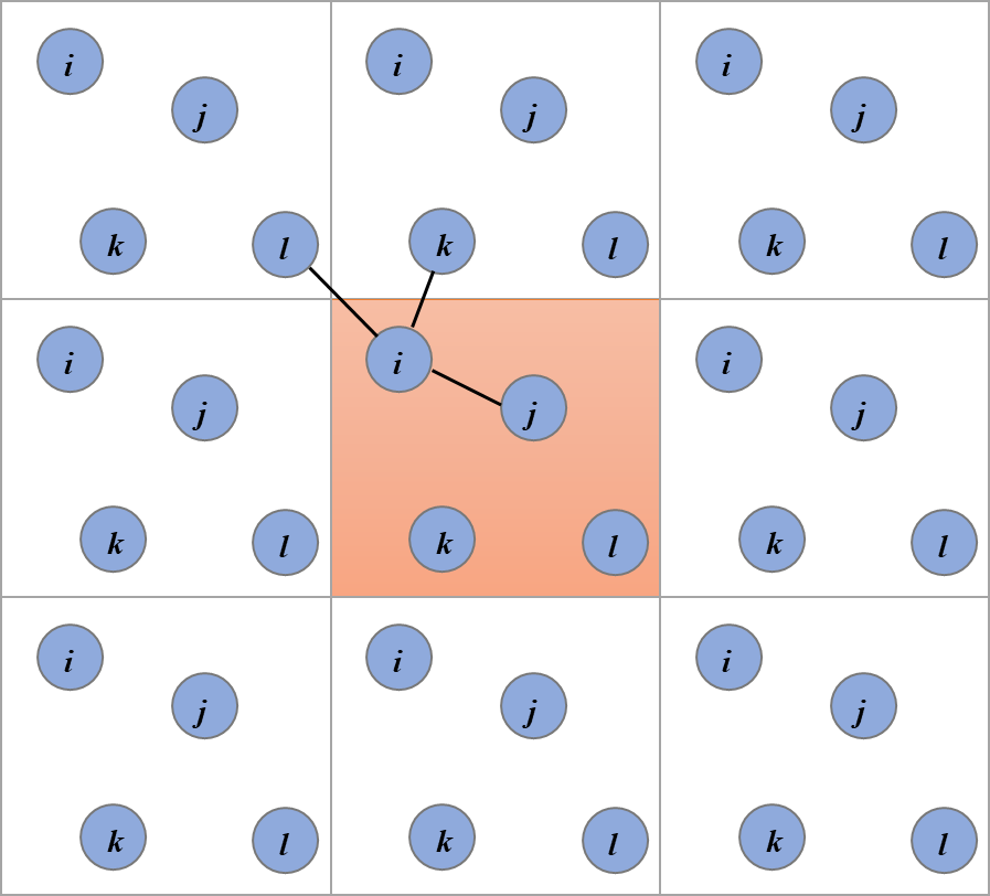
Figure 1:A schematic representation of periodic-boundary conditions and the minimum-image construction for a two-dimensional system. The system shown here contains 4 particles (labelled , , , and ), with the black lines connecting particle with the closest periodic images of the other particles. Credits to Abusaleh AA via Wikimedia Commons.
The total force acting on a particle can now be computed by summing up the contributions due to each particle , where the distance is given by Eq. (13).
The use of periodic boundary conditions gets rid of surface effects altogether, and more generally can greatly limit finite-size effects, even for small numbers of particles. However there are some important things that should always be kept in mind when using PBCs (which is by far the most common form of boundary conditions employed in molecular simulations):
If the system under study exhibit correlations that are of the same order of or exceed the box size, the system will “feel itself” through the PBCs, leading to spurious non-linear effects.
Only wavelengths compatible with the box size are allowed. This is true for any observable, and applies to a wide range of phenomena. For instance
If one wishes to simulate equilibrium crystals, the shape of the box and the length of its sides should be compatible with the lattice’s unit cell.
Fluctuations with wavelengths longer than the box size are suppressed. This makes it hard to study critical phenomena, which have diverging correlation lengths.
Angular momentum is not conserved, since the system is not rotationally invariant (even if the Hamiltonian is).
When particles cross the box boundary to, for instance, exit the central cell, one of its images will enter it. It is important to keep track of the “original” particle to correctly compute the value of some observables (e.g. the mean-squared displacements, see below, or chain connectivity).
1.4Integrating the equations of motion
Consider a particle moving along the -axis under the influence of a force . Newton’s second law gives , so that the acceleration .
Expanding the position around using a Taylor series we obtain
Adding the two Taylor expansions yields
which, if we neglect the higher-order terms becomes
This is the Verlet algorithm, which allows us to calculate the position at the next time step using the current position , the previous position , and the current acceleration . Although this basic Verlet method does not explicitly involve velocity, if we consider the expansion up to the second order we can explicitly write
Note the lower order of accuracy with respect to . We can modify the basic Verlet approach to include an explicit update for the velocity, leading to the Velocity Verlet method. Instead of relying on the positions from the previous and current time steps, the Velocity Verlet algorithm updates the position and velocity in a two-step process.
First, we use the current velocity and acceleration to update the position at time . This is done similarly to the basic Verlet method but with the velocity term explicitly included:
This equation uses the current position , the current velocity , and the current acceleration to compute the new position . Next, after updating the position, we need to compute the new acceleration at time because the force (and hence the acceleration) has changed due to the updated position. The new acceleration is given by:
With this new acceleration in hand, we can update the velocity. Instead of using just the current acceleration, the Velocity Verlet method uses the average of the current and new accelerations to update the velocity:
This velocity update equation accounts for the change in acceleration over the time step, providing a more accurate velocity update than simply using the current acceleration. The Velocity Verlet method is the de-facto standard for MD codes. The common way to implement it is to split the velocity integration step in two, so that a full MD interation becomes
Update the velocity, first step, .
Update the position, (e.g. Eq. (18)).
Calculate the force (and therefore the acceleration) using the new position, .
Update the velocity, second step, (e.g. Eq. (20)).
An MD implementation based on Program 1 that implements a Velocity Verlet algorithm is
CALL initialise_parameters()
CALL initialise_system()

WHILE t is smaller than t_max
   CALL integrate_first_step()
   CALL compute_force()
   CALL integrate_second_step()

   t += delta_t
   CALL sample_observables()
Program 2:Pseudo-code for an MD code implementing the Velocity Verlet algorithm.
1.5Energy conservation
The Velocity Verlet algorithm is symplectic, which means that it conserves the energy (i.e. the value of the Hamiltonian)[5]. This is not a common property, as most schemes (such as the explicit Euler scheme or the famous Runge-Kutta method) are not symplectic, and therefore generate trajectories that do not live on the hypersurface. Since this is where the dynamics of systems evolving through Newton’s equations move, MD integrators should always be symplectic. If this is the case, the resulting molecular dynamics simulations will conserve the total energy, which is a constant of motion. In turn, this means that MD simulations sample the microcanonical ensemble (as long as the system is ergodic, so that time and ensemble averages are equivalent).
Since we are discretising the equations, there are two caveats associated to the energy conservation:
If the time step is too large, then a deviation (drift) from the “correct” value of the energy will be observed. A good rule of thumb to avoid an energy drift, which would invalidate the simulation, is to calculate the highest vibrational frequency associated to the interaction potential employed, , where is the highest curvature of the potential, i.e. the largest value of , and is the mass of the particle. Then, a sensible value for the integration time step is an order of magnitude less than the characteristic time associated to , i.e. .
If the value of is appropriate, then the energy will be conserved on average, meaning that it will fluctuate around its average value with an amplitude, . If the integrator is of the Verlet family (i.e. Velocity Verlet), then . This behaviour can be exploited to ensure that codes and simulations are working correctly, at least from the point of view of the energy conservation. See Figure 2 for an example.
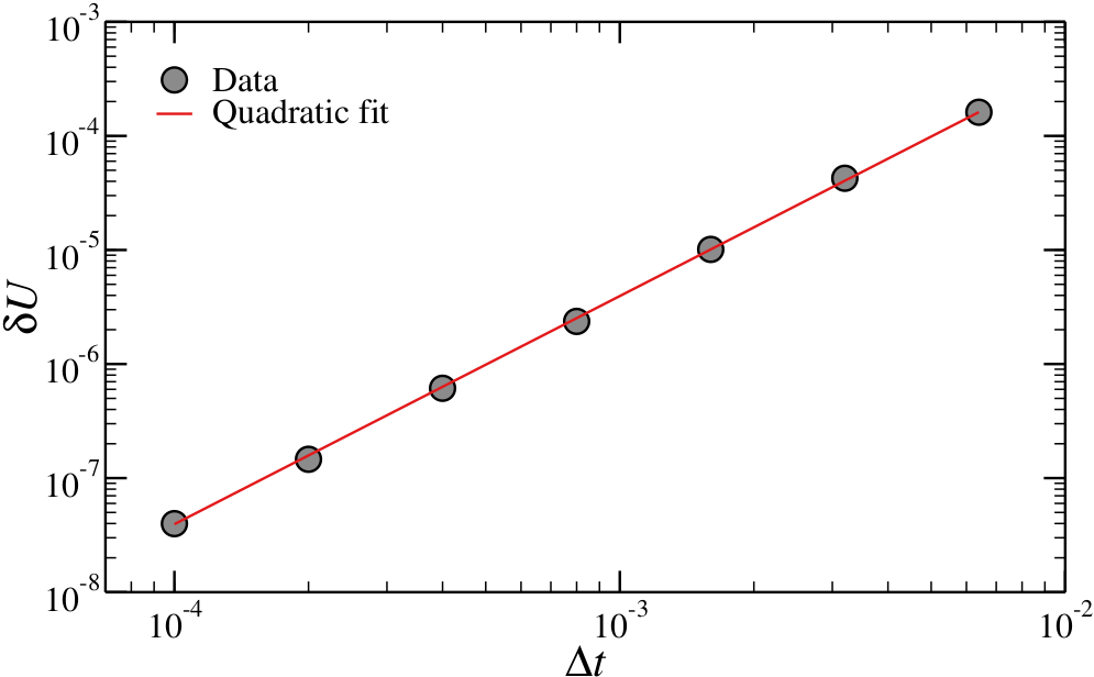
Figure 2:The extent of the fluctuations of the total energy, , for a Lennard-Jones system simulated at and as a function of the time step . The line is a quadratic fit. Nota Bene: this scaling requires that truncation errors are small, which is why I had to use a rather large cut-off, .
1.6Some observables
Since, in principle, we have access to the whole phase space, in MD simulations we can compute averages of any (classical) observable. Here I present a short list of some useful (and common) quantities.
1.6.1Pressure
In the canonical ensemble, for any observable and generalised coordinate or momentum , integrating by parts (and assuming reasonable boundary conditions) one finds
which translates to the following generalised equipartition relation:
If we plug in a generalised momentum and sum over all momenta, Eq. (22) yields the usual equipartition principle:
By contrast, if we choose to use Cartesian coordinates as generalised coordinates in Eq. (22) and recall that the derivative of the Hamiltonian with respect to a particle coordinate is minus the total force acting on the particle along that coordinate, we find
where is the position of particle . Note that here is the sum of inter-molecular interactions, , and external forces, . If the latter consist only of the forces exerted by the container walls (which keeps the system in a volume under a pressure ), we have
Since , we find
where I have defined the instantaneous pressure . The second term in Eq. (26) represents the contribution from interparticle forces, where is the force on particle due to all other particles. Applying Eq. (26) makes it possible to evaluate the pressure in computer simulations.
1.6.2Radial distribution function
The simplest, and most straightforward, piece of structural information that can be extracted from simulation output is encoded in the pair correlation function, also known as the radial distribution function, .
Let us start by defining a function such that represents the number of particles found between and , assuming the origin is placed at a random particle. With this definition, the total number of particles contained within a sphere of radius centered on a random particle is:
For an ideal gas, , where is the number density .
The function is defined as:
and it indicates how much denser the system is at a distance compared to an ideal gas. The function is always positive and, for large values of , . The is a central observable in molecular simulations, as it can be used to estimate many other quantities (see e.g. Hansen & McDonald (2013)).
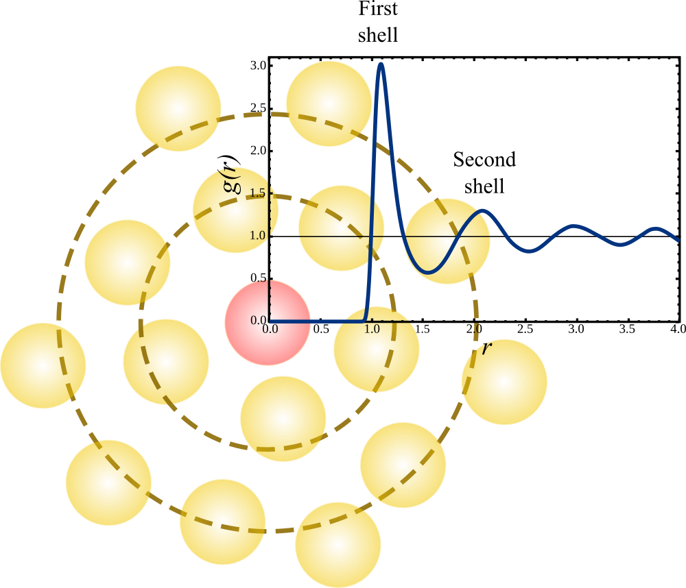
Figure 3:The radial distribution function of a Lennard-Jones fluid at and . Superimposed on the plot is a cartoon that shows the interpretation of the features of the , highlighting the first and second shells around the central particle (coloured in red). Adapted from Wikipedia.
Figure 3 shows a typical shape of , together with a 2D cartoon that gives an idea of how the structural features of the system determine the resulting radial distribution function. Near the origin, due to the excluded volume. This is always observed in simple liquids and, more generally, in systems with short-range repulsions (such as atom-based systems). For soft (or ultrasoft) potentials, which are typically effective, may not be zero even at the origin.
Figure 3 also conveys a second message: the packing of objects with excluded volume inevitably generates oscillations in the function, with a periodicity determined by the diameter of the particles themselves.

Figure 4:The (a) and (b) radial distribution functions of SPC/E liquid water at C. Taken from Svishchev & Kusalik (1993).
In a system composed by atoms (or particles) of different types, it is possible to define radial distribution functions between pairs of atom types. For instance, when simulating water it is common to define , , and , which provide information on the oxygen-oxygen, hydrogen-hydrogen and hydrogen-oxygen pair correlations, respectively. See Figure 4 for an example.
1.6.3Mean-squared displacement
The mean squared displacement (MSD) quantifies the extent of particle diffusion within a system over time. It provides insights into the mobility of particles by tracking how far each particle moves from its original position. Formally, for a given particle , the MSD at time is calculated as the average of the squared differences between its position at that time and its initial position , represented as , so that the overall MSD is
In MD simulations, the MSD can be computed by first recording the position of each particle at each timestep, then calculating the squared displacement for each particle relative to its starting position, and finally averaging this value over all particles. If the system is ergodic, as it is often the case, we can also average over different time origins to decrease the statistical error. This is done by averaging contributions of the type for multiple values of .
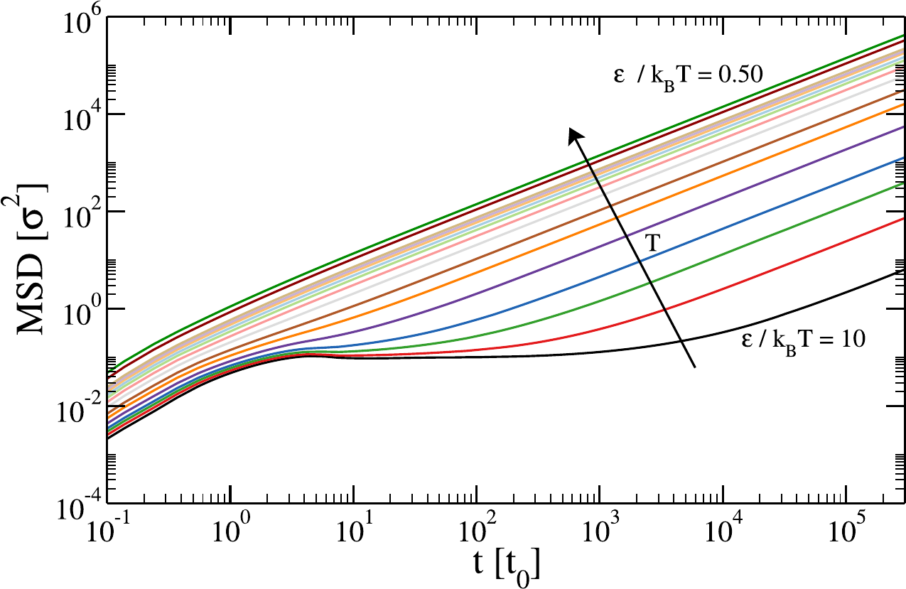
Figure 5:The mean-squared displacement of a coarse-grained system (a tetravalent patchy particle model) computed at fixed density and varying ratio between the attraction strength (kept constant) and the thermal energy, . Taken from Gomez & Rovigatti (2024).
The MSD provides essential information on diffusive behavior, as its time dependence can help distinguish between different diffusion regimes, such as ballistic (), brownian (), or subdiffusive (e.g. , with < 1), which are characteristic of different types of material and dynamical properties. Figure 5 provides an example of a system that, depending on temperature, experience all these regimes.
1.6.4Root mean-squared deviation
The root mean-squared deviation (RMSD) is a measure commonly used to assess the structural deviation of a molecule or a set of particles from a reference structure, typically the initial or an experimentally determined structure. It quantifies the average distance between corresponding atoms in two structures, giving insight into conformational changes over time. The RMSD is particularly useful in studying the stability and flexibility of molecular structures, such as proteins, over the course of a simulation.
Formally, for a system with atoms, the RMSD at time relative to a reference structure is given by:
where is the position of the -th atom in the reference structure. To compute the RMSD in MD simulations, Eq. (30) is evaluated after the configuration at time is aligned with the reference structure (typically minimizing rotational and translational differences). Formally, this can be written as
where and are the rotation matrix and translation vector that minimise the resulting RMSD, respectively. The most common use of the RMSD is to plot it as a function of time to analyse the stability of the molecule: lower RMSD values indicate that the structure remains close to the reference, while higher values suggest significant conformational changes. It is rather common to only use a subset of atoms to compute the RMSD (e.g. to compare the structure of two polypeptides with different sequences, only backbone atoms are used).
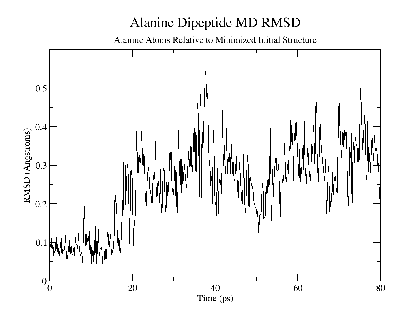
Figure 6:The RMSD of a Alanine dipeptide simulated with Amber. Taken from this Amber tutorial.
Figure 6 shows the RMSD of a simulation of a small molecule (an Alanine dipeptide). In this example the small value of the RMSD throughout the trajectory shows that there is no significant conformational change in the positions of the atoms relative to the starting structure.
1.7Tricks of the trade
1.7.1Neighbour lists
If the interaction potential is short-ranged, in the sense that it goes to zero at some distance , it is clear that particles that are further away than will not feel any reciprocal force. If this is the case, calculating distances between all pairs of particles would be wasteful, as only a fraction of pairs will feel a mutual interaction. There are several techniques that can be used to optimise the force calculation step (and therefore the simulation performance) by performing some kind of bookkeeping that makes it possible to evaluate only those contributions due to pairs that are “close enough” to each other. Here I will present the most common ones: cells and Verlet lists.
The idea behind cell lists is to partition the simulation box into smaller boxes, called cells, with side lengths [6]. This partitioning is done by using a data structure that, for each cell, stores the list of particles that are inside it. Then, during the force calculation loop, we consider that particle , which is in cell , can interact only with particles that are either inside or in one of its neighbouring cells (8 in 2D and 26 in 3D). The cell data structure can either be built from scratch every step, or updated after each integration step. In this latter case, the code checks whether a particle has crossed a cell boundary, and in this case it removes the particle from the old cell and adds it to the new one. This can be done efficiently with linked lists. With this technique, each particle has a number of possibly-interacting neighbours that depends only on particle density and cell size, and therefore is independent on . As a result, the algorithmic complexity of the simulation is rather than .
Differently from cell lists, with Verlet lists the code stores, for each particle, a list of particles that are within a certain distance , where is a free parameter called “Verlet skin”. Every time the lists are updated, the current position of each particle , is also stored. During the force calculation step of particle , only those particles that are in ’s Verlet list are considered. For a homogeneous system of density , the average number of neighbours is
which should be compared to the average number of neighbours if cell lists are used, which in three dimensions is
In the limit , which is rather common, , so that : with Verlet lists, the number of distances to be checked is six times smaller than with cell lists.
Verlet lists do not have to be updated at every step, or we would go back to checking all pairs, but only when when any particle has moved a distance larger than from its original position . Note that the overall performance will depend on the value of , as small values will result in very frequent updates, while large values will generate large lists, which means useless distance checks on particles that are too far away to interact. Although the average number of neighbours of each particle is independent on and therefore the actual force calculation is , the overall algorithmic complexity is still , since list updating, even if not done at each time step, requires looping over all pairs. To overcome this problem it is common to use cell lists to build Verlet lists, bringing the complexity of the list update step, and therefore of the whole simulation, down to , while at the same time retaining the smaller average number of neighbours of Verlet lists.
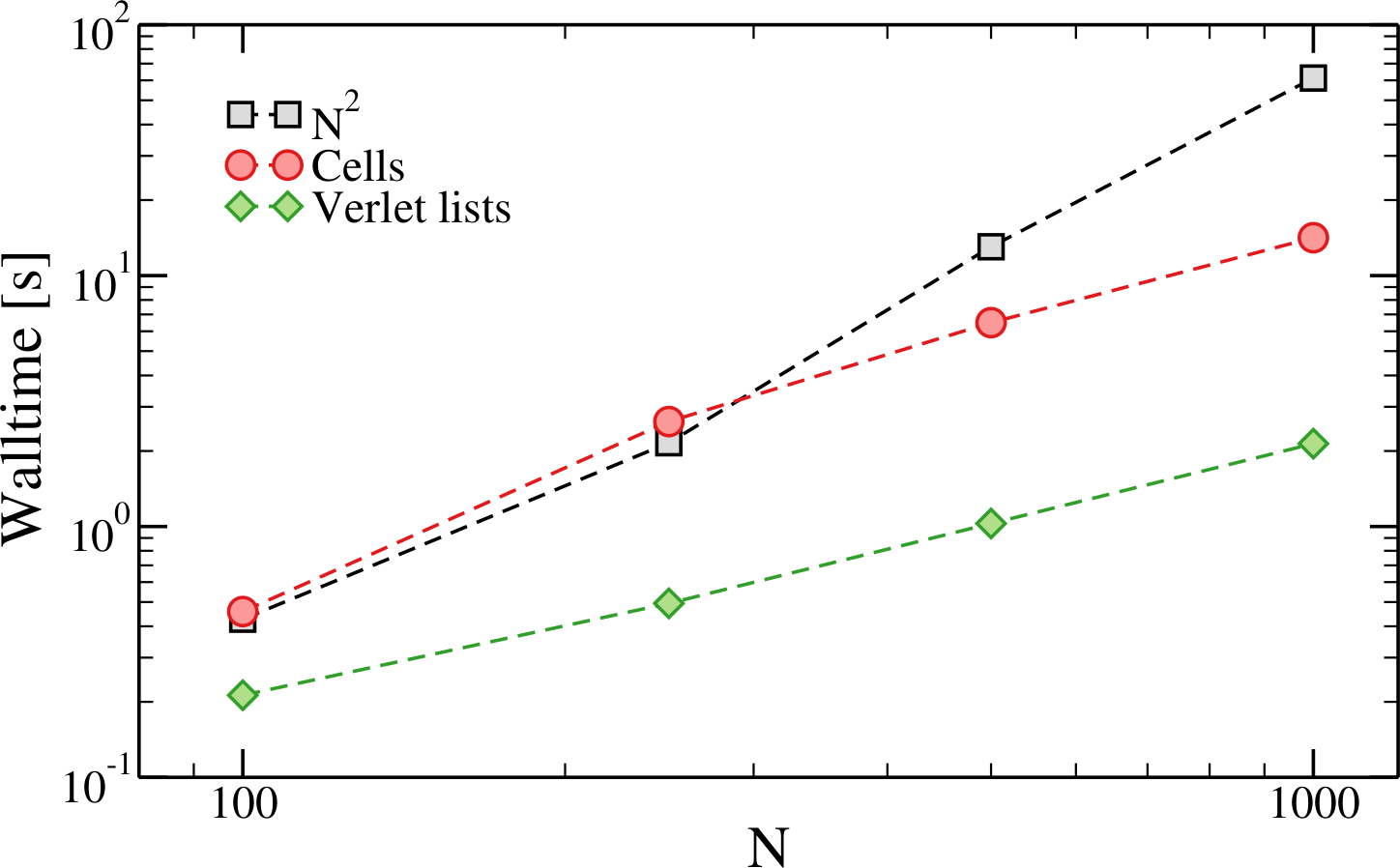
Figure 7:The time taken to run 10000 MD steps of LJ systems with and varying number of particles with and without neighbouring lists. These simulations have been run with oxDNA.
Figure 7 shows that, as soon as the number of particles is great enough ( for most MD codes), the overhead due to the additional bookkeeping required to implement neighbour lists is dwarfed by the scaling of the trivial approach. The figure also shows the speed-up that can be achieved with Verlet lists.
1.7.2Long-range interactions
In molecular simulations, long-range interactions refer to forces that decay slowly with distance. The definition of “long-range” can be made unambiguous if we consider the general form of a pairwise interaction potential between two particles separated by a distance . The energy contribution of these interactions beyond a certain cut-off distance is given by the “tail” correction defined in Eq. (7). For a potential that decays as , the tail correction in 3D is, asymptotically,
which converges for any as long as (e.g. the Lennard-Jones potential, for which )[7]. By contrast, if , the integral diverges, indicating that the tail of the interaction potential beyond contributes non-negligibly to the total energy of the system regardless of the value of , making a direct cut-off inaccurate.
I’ll now quickly introduce the most popular methods used to handle long-range interactions, together with two techniques used to improve its efficiency. First, we start by considering a system consisting of charged particles in a box of volume and periodic boundary conditions. We assume that particles cannot overlap (i.e. that there is at least an additional short-range repulsion), and that the system is electrically neutral, e.g. that . The total electrostatic energy of the system (in Gaussian units, which make the notation lighter) is
where the prime on the summation indicates that the sum is over all periodic images and over all particle pairs , except if , i.e. particle interacts with all its periodic images but not with itself. Unfortunately, Eq. (35) cannot be used to compute the electrostatic energy in a simulation because it contains a conditionally convergent sum.
To improve the convergence of the expression for the electrostatic potential energy, we follow Ewald (1921) and rewrite the expression for the charge density. In equation (35) the charge density is represented as a sum of -functions. The contribution to the electrostatic potential due to these point charges decays as . Now consider what happens if we assume that every particle with charge is surrounded by a diffuse charge distribution of the opposite sign, such that the total charge of this cloud exactly cancels . In that case only the fraction of that is not screened contributes to the electrostatic potential due to particle . At large distances, this fraction goes to 0 in a way that depends on the functional form of the screening charge distribution, which we will take as Gaussian in the following.

Figure 8:The elecrostatic effect due to point charges can be seen as a sum of screend charges, minus the smoothly varying screening background. Taken from Frenkel & Smit (2023).
The contribution to the electrostatic potential at a point due to a set of screened charges can be easily computed by direct summation, because the electrostatic potential due to a screened charge is a rapidly decaying function of . However, we must correct for the fact that we have added a screening charge cloud to every particle. This is shown schematically in Figure 8. This compensating charge density varies smoothly in space (because the screening charge distribution is a smoothly varying function!). We now wish to compute the electrostatic energy at the site of ion . Of course, we should exclude the electrostatic interaction of the ion with itself. We have three contributions to the electrostatic potential: first of all, the one due to the point charges , secondly, the one due to the Gaussian screening charge clouds with charge , and finally the one due to the compensating charge clouds with charge . In order to exclude Coulomb self-interactions, we should not include these three contributions with to the electrostatic potential at the position of ion . However, it turns out that it is convenient to retain the contribution due to the compensating charge distribution and correct for the resulting spurious interaction afterwards. The reason we retain the compensating charge cloud for ion is that, if we do so, the compensating charge distribution is not only a smoothly varying function, but it is also periodic. Such a function can be represented by a (rapidly converging) Fourier series, and this turns out to be essential for the numerical implementation. Of course, in the end we should correct for the inclusion of a spurious “self” interaction between the ion and the compensating charge cloud.
Considering screening Gaussians with width , the splitting can be written as follows:
where is a parameter that controls the width of the Gaussian distribution used to split the potential, and and are the complementary error function and error function, respectively, and they come out from integrating the Gaussian screening function. In Eq. (36), the first term decays quickly as increases, so it is computed only for nearby particles within a cut-off . By contrast, the second term decays slowly in real space, but can be computed efficiently in Fourier space, using a sum over reciprocal lattice vectors , which can be again truncated beyond a cut-off wavevector .
The total electrostatic energy using Ewald summation is the sum of the real-space term, the reciprocal-space term, and the self-interaction correction:
The real-space contribution to the total energy, is given by:
where the sum is truncated at the cut-off distance .
The reciprocal-space contribution is computed using the Fourier transform of the charges and involves a sum over the reciprocal lattice vectors :
where the sum can be safely truncated at some cut-off wavevector , since the exponential term ensures that the sum converges rapidly.
The self-interaction term, , is:
Note that there are many subtleties that are linked to the boundary conditions that are applied to the system (even though the latter is infinite!). Have a look at Frenkel & Smit (2023) and Schlick (2010) (and references therein) for additional details.
For fixed values of and , the algorithmic time scales as . However, this behaviour can be improved by realising that there are values of the cut-offs that minimise the error due to the truncations. Using these values, that depend on , the complexity can be brought down to .
A further scaling improvement can be obtained by using the so-called Particle Mesh Ewald method (Darden et al. (1993)). In the PME method, the basic idea is to use Poisson’s equation to compute the potential. Indeed, Poisson’s equation can be easily solved in Fourier space, where it takes the form
where is the Fourier transform of . Leveraging Eq. (41), in the PME method the reciprocal space contribution to electrostatic interactions is computed through the following series of steps that involve transforming particle charges into a charge density on a grid, applying Fourier transforms, and then transforming back to obtain the forces and energies:
Assign each particle’s charge to a regular 3D grid that spans the simulation box. This is achieved through an interpolation scheme, where each particle’s charge is “spread” over multiple neighboring grid points. The most common method is B-spline interpolation (see Essmann et al. (1995) for details).
Once the charges are mapped onto the grid, the Fourier transform of the grid-based charge density is computed. This is done by using the Fast Fourier Transform (FFT), an efficient algorithm for performing discrete Fourier transforms, with a computational complexity of .
In Fourier space, the electrostatic potential for each grid point at wave vector is computed by first applying the Ewald screening function (i.e. Eq. (39)) to obtain the charge density, and then solving the Poisson equation.
Once the reciprocal-space potential has been calculated, an inverse Fourier transform is applied to convert the potential back to real space on the grid, yielding the electrostatic potential on each grid point in the simulation box.
The final step is to interpolate the grid-based potential back to the positions of the actual particles, which allows the forces and energies to be computed for each particle based on the smoothed potential field. This is essentially the reverse of the initial charge assignment process, with each particle’s force interpolated from the neighboring grid points.
If the cut-off of the real-space contribution is chosen so that can be computed in , the overall complexity of the PME method is , which is much better than . The method has some constant overhead that makes it slower than the original Ewald sums only for small systems, which is why PME is the de-facto standard of biomolecular simulations.
Note that it is possible to achieve linear scaling () using sophisticated techniques such as the Fast Multipole Method (see e.g. Greengard & Rokhlin (1987), but those are rather difficult to implement, and not widely used yet.
2Other ensembles
We know from statistical mechanics that, in the thermodynamic limit, all ensembles are equivalent. However, in simulations it can be convenient to use different ensembles, depending on the phenomena one wishes to study. I will now briefly present some methods that can be used to fix the temperature (rather than energy) and the pressure (rather than volume) in MD simulations.
2.1Thermostats
Before introducing some of the schemes that are used to perform Molecular Dynamics simulations at constant temperature, it is important to understand what “constant temperature” even means. From a statistical mechanical point of view, there is no ambiguity: we can impose a temperature on a system by bringing it into thermal contact with a large heat bath. Under those conditions, the distribution of the velocities is given by the Maxwell-Boltzmann distribution (Eq. (4)), whose second moment is connected to the temperature via Eq. (2). Given in this form, it is clear that the temperature also fluctuates, with the fluctuations being linked to the second and fourth moment of the Maxwell-Boltzmann distribution (e.g. ). Therefore, any algorithm devised to fix the temperature of a MD simulation should reproduce not only the average , but also its fluctuations. Here I will present three such algorithms.
2.1.1Andersen
The Andersen thermostat is a widely used method in molecular dynamics simulations for controlling temperature, introduced by Hans C. Andersen in 1980. Its fundamental idea is to maintain a system’s temperature by coupling the particles to an external heat bath through random collisions. In this approach, particles in the simulation periodically undergo stochastic collisions with a fictitious heat bath, resulting in velocity reassignment according to a Maxwell-Boltzmann distribution that corresponds to the desired temperature. This random reassignment of velocities, which can be considered as a Monte Carlo move that transports the system from one constant-energy shell to another, mimicking the effect of a thermal reservoir, ensuring that the system reaches and maintains thermal equilibrium.
The thermostat has a parameter that is the frequency of stochastic collisions, which represents the strength of the coupling to the heat bath: by adjusting this collision frequency, the user can control how frequently the system interacts with the heat bath, thus influencing the rate at which the system equilibrates. In practice, at each time step each particle has a probability of undergoing a collision, i.e. of being reassigned a velocity from a Maxwell-Boltzmann distribution corresponding to the target temperature. This scheme reproduced the canonical ensemble, since temperature fluctuations align with those expected from statistical mechanics.
One drawback of the Andersen thermostat is connected to its stochastic nature: the random collisions “disturb” the dynamics in a way that is not realistic. In particular, they enhance the decorrelation of the particle velocities, thereby affecting quantities such as the diffusion constant. This effect depends on the value of : the larger the collision frequency, the faster the decorrelation, the smaller the diffusion constant. Therefore, the Andersen thermostat should be used when we are interested in static properties only, and dynamics observables are not important.
2.1.2Nose-Hoover
The Nosé-Hoover thermostat is a more sophisticated method for controlling temperature in molecular dynamics simulations, designed to generate the canonical ensemble while preserving the continuous evolution of the system’s dynamics. Unlike the Andersen thermostat, which introduces stochastic velocity reassignment, the Nosé-Hoover thermostat operates deterministically by coupling the system to a fictitious heat bath via an extended Lagrangian formalism. This allows the system to exchange energy with the thermostat in a smooth and continuous manner, maintaining temperature without introducing artificial randomness.
The extended Lagrangian formalism starts by introducing a scaling factor, , that modifies the velocities of particles in the system (Nosé (1984)). The extended Lagrangian for the Nosé-Hoover thermostat is expressed as:
where and are the mass and velocity particle , is the potential energy of the system, and the term , where is the number of degrees of freedom, introduces the necessary coupling between the system and the heat bath. The auxiliary variable is responsible for controlling the temperature by scaling the velocities of the particles so that the system’s kinetic energy corresponds to the target temperature.
The dynamics of the system are then derived from this Lagrangian. The equations of motion for the positions and velocities of the particles are modified by the thermostat, resulting in:
where is the force acting on particle , and the term is a friction-like coefficient that emerges from the thermostat variable. This friction term adjusts the particle velocities in response to deviations from the target temperature, ensuring that the system remains at the correct thermal equilibrium, and evolves according to:
where is a parameter that controls the strength of the coupling between the system and the thermostat, is the momentum conjugate to , so that is the total kinetic energy of the system, and represents the target thermal energy. If the system’s kinetic energy exceeds the desired value, the variable increases, effectively damping the particle velocities to bring the temperature back in line. Conversely, if the kinetic energy is too low, decreases, allowing the velocities to rise and the temperature to stabilize at the target value. The “inertia” of this process is controlled by the value of , which therefore plays the role of a fictitious mass. This deterministic feedback mechanism distinguishes the Nosé-Hoover thermostat from stochastic approaches. By continuously adjusting the velocities of all particles, this method preserves the natural evolution of the system’s dynamics while still achieving temperature control. The benefit of using this extended Lagrangian framework is that it allows for smooth, continuous temperature regulation without disrupting important dynamical properties, such as diffusion coefficients or time-dependent correlations.
Note that the above equations of motion conserve the following quantity
which can be used as a check when implementing the thermostat, or when testing the simulation parameters (e.g. the time step). Hoover (1986) demonstrated that the above equations of motion are unique, in the sense that different equations of the same form (i.e. containing an additional friction-like parameter) cannot lead to a canonical distribution. However, the simulation samples from the canonical distribution only if there is a single non-zero constant of motion, the energy. If there are more conservation laws, which can happen, for instance, if there are no external forces and the total momentum of the system is different from zero, than the Nosé-Hoover method does not work any more.

Figure 9:The trajectory of the harmonic oscillator for a single initial condition simulated (from left to right) without a thermostat, with the Andersen thermostat, with the Nosé-Hoover thermostat. Adapted from Frenkel & Smit (2023).
Figure 9 shows the failure of this thermostat for a cases that is deceptively simple: that of a harmonic oscillator. It is obvious that the dynamics simulated in the microcanical ensemble or with the Nosé-Hoover thermostat becomes non-ergodic. Although in practice one can always set the initial velocity of the centre of mass of the system to zero to remain with a single non-trivial conserved quantity and therefore avoid this issue, it would be better to have an algorithm that works well in the general case[8].
As demonstrated in Martyna et al. (1992), this issue can be overcome by coupling the Nosé-Hoover thermostat to another thermostat or, if necessary, to a whole chain of thermostats, which take into account additional conservation laws. Here I provide the equations of motion for a system coupled to an -link thermostat chain, where each link is an additional degree of freedom associated to a “mass” :
As discussed in Frenkel & Smit (2023) (where all these arguments are presented more in depth) of the additional degrees of freedom only two (the first link and the thermostat “centre”, ) are independently coupled to the dynamics, which is what is needed when there are two conservation laws.
2.1.3Bussi-Donadio-Parrinello
We know from the equipartition theorem, Eq. (2), that the instantaneous temperature is related to the kinetic energy of the system, , through:
Since on a computer we always have a discrete dynamics, in the following I will slightly abuse the notation by using to mean , where is an index that keeps track of the time step and is a time-dependent function.
The simplest way of fixing the temperature is to scale the velocities to achieve the target temperature instantaneously: the new velocities are obtained from the old velocities by multiplying them by a scaling factor , e.g. , where is given by
where and are the target temperature and kinetic energy. This method has two drawbacks:
It does not yield the correct fluctuations for the kinetic energy.
The rescaling affects all particles at the same time in a abrupt way, greatly disturbing the dynamics, as was the case with the Andersen thermostat.
The second issue can be mitigated by weakly coupling the system to a heat bath with a characteristic relaxation time . With this method, called the Berendsen thermostat, the velocities are gradually adjusted to bring the temperature toward the target value. The velocity scaling factor in the Berendsen thermostat is given by:
This factor ensures that the system’s temperature approaches over time, with the relaxation time controlling the speed of this adjustment. The Berendsen thermostat achieves smooth temperature control, but it still suppresses the natural energy fluctuations required for proper sampling of the canonical ensemble.
Bussi et al. (2007) introduced a thermostat that is based on the idea of velocity rescaling, but it samples the canonical ensemble. Note that in the continuous limit, i.e. for , Eq. (49) becomes[9]
This equation makes it obvious that exponentially, in a deterministic way (i.e. without fluctuations). A way of introducing fluctuations is to add a Weiner noise , weighted by a factor that ensures that the fluctuations of the kinetic energy are canonical[10]:
where is the number of degrees of freedom in the system. Since the total momentum is conserved, in a 3D simulation. With some non-trivial math Bussi et al. (2007) demonstrated that Eq. (51) yields the following scaling factor:
where the are independent random numbers extracted from a Gaussian distribution with zero mean and unit variance.
The interpretation of Eq. (51) is that, in order to sample the canonical ensemble by rescaling the velocities, the target kinetic energy (i.e. the target temperature) should be chosen randomly from the associated canonical probability distribution function[11]:
One way of doing this would be to randomly extract a value from Eq. (53) each time a rescale should be performed, and use it as the target kinetic energy in Eq. (48). However, this would generate abrupt changes in the dynamics, as for the simple velocity rescaling and Andersen thermostats. By contrast, the stochastic process defined in Eq. (51) is smoother, since the rescaling procedure happens on a timescale given by , in the same vein as with the Berendsen thermostat.
As for the Nosé-Hoover thermostat, this thermostat, which is sometimes called the stochastic velocity rescaling thermostat, has an associated conserved quantity that can be used to check the choice of the time step and of the other simulation parameters:
2.1.4Other thermostats
There are many other thermostats, which I will not introduce here because of time constraints. Here I list a few, just for reference:
Langevin thermostats for systems where the dynamics is overdamped. Examples are particles dispersed in a viscous fluid.
Brownian thermostats for systems where inertia is negligible. Examples are concentrated suspensions of colloids or bacteria.
Stochastic rotational dynamics to model hydrodynamic interaction. Examples are diluted solutions of colloids or bacteria where long-range hydrodynamic effects are important and of interest (e.g. sedimentation or flocking).
2.2Barostats
Experiments are usually performed at constant pressure (e.g. ambient pressure). Moreover, while statistical mechanics results ensure that ensembles are equivalent in equilibrium, there are many situations in which it is more convenient to simulate in a specific ensemble. For instance, equilibrating a crystal structure usually requires that the edge lengths of the box can relax and fluctuate, or the coexisting region between a gas and a liquid is extended in , but it is just a line in the projection. Just like controlling the temperature requires coupling the system to a thermostat, fixing means coupling the system to a barostat. When simulating at constant pressure it is very common, but by no means the only possibility, to also fix the temperature, thereby simulating in the so-called isothermal-isobaric ensemble.
As for thermostats, there exist many barostats, each having its own unique advantages and disadvantages. Here I briefly present three barostats, two based on the extended-Lagrangian formalism and a stochastic one.
2.2.1Nosè-Hoover (MTTK) barostat
The Nosè-Hoover formalism can be extended to fix the pressure in addition to temperature. In this case the equations of motion for a system coupled to a barostat and to a single Nosé-Hoover thermostat, as presented in Martyna et al. (1994), which improves the original scheme by Hoover that only yields approximated constant- distributions, are:
where is the volume of the simulation box, is the space dimensionality, , where is the volume at , is the inertia parameter associated to , is the conjugate momentum of (here I’m using the same notation as Frenkel & Smit (2023)), and and are the target and instantaneous pressures, respectively. In particular, the instantaneous pressure is
which is the virial pressure of a system with a non-constant volume. Note that the second term in (56) is non-zero if the energy depends explicitly on volume, which is always the case for interaction potentials that are long-range, or for which long-range corrections due to cut-offs have to be evaluated.
Note that equations (55) also contain a coupling to a Nosé-Hoover thermostat, which can be generalised to a chain thermostat if , , and the equations of motions of the other links are added.
2.2.2Parrinello-Rahman
The Parrinello-Rahman barostat, introduced in Parrinello & Rahman (1980), uses an extended Lagrangian to account for both particle motions and cell shape fluctuations, enabling the simulation of anisotropic pressure conditions, which is very common, for instance, when dealing with crystalline structures. This Lagrangian includes the original Lagrangian of the system, which accounts for the kinetic and potential energy of the particles, plus additional terms that describe the kinetic and potential contributions of the simulation box itself.
The additional terms can be written in terms of the matrix
where , and are the basis vectors of a generic (possibly anisotropic) simulation box, and coincide with its edges. The position of particle in the box is just
where are the scaled (fractional) coordinates of particle . With this formalism, the distance between particles and is
where .
We can now write down the expression for the extended Lagrangian:
where , is the target pressure, and the parameter is the strength of the barostat coupling, which can be interpreted as the mass of the fictitious piston exerting the external pressure on the system.
By deriving Eq. (60), the following equations of motion are obtained:
2.2.3Stochastic cell rescaling
3All-atom force fields
Now that we know the algorithms used to run MD codes, we shift our attention to the interaction potentials acting between the components that make up the system we want to simulate. We start from the so-called classical (or empirical) force fields, which describe the interactions between atoms using simplified mathematical models based on quantum mechanics calculations, empirical observations, and physical principles from classical mechanics. Unlike quantum methods (introduced in Molecular quantum mechanics), which rigorously account for the wave-like nature of particles and their interactions through principles like superposition and entanglement, classical force fields offer a pragmatic approach that balances computational feasibility with accuracy.
The potential energy functions used in classical force fields typically consist of terms that describe various types of interactions, including covalent bonds, van der Waals (dispersion) forces and electrostatic interactions. Despite their simplicity, classical force fields can exhibit remarkable predictive power and have been successfully applied across diverse scientific disciplines. Common force fields used in biomolecular simulations are AMBER and CHARMM.
In a classical force field (FF from now on), the main assumption is that of additivity, which makes it possible to write down the total energy of a system as a sum of several contributions. These are classified into terms that account for atoms that are linked by covalent bonds (bonded or local terms), and terms that account for noncovalent interactions (non-bonded or non-local terms), so that the total energy of the system is written as
where I made explicit the fact that the energy (and its contributions) are functions of the set of positions of the atoms, .
The functional forms of the functions (implicitly) defined in Eq. (62) depend on the force field employed, and are parametrised so as to reproduce the experimental structure and dynamics of target molecular systems, but also leveraging ab initio calculations, which are often used to complement the experimental results.
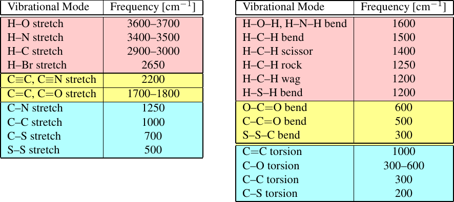
Figure 10:Characteristic (left) stretching and (right) bending and torsional vibrational frequencies extracted from experimental spectra. Taken from Schlick (2010).
The traditional sources of parameters are provided by vibrational spectra (see Figure 10 for examples), which have been routinely used to derive the force constants of many of the functional forms discussed below. The idea is that the frequencies extracted from experimental spectra can be compared with the characteristic frequencies of the normal modes as evaluated in simulations in order to find the values of the force constants that minimise the differences.
3.1Bonded interactions
In the context of molecular systems, bonded interactions refer to the forces that arise between atoms due to the formation of chemical bonds. These interactions occur when atoms are directly connected to each other through covalent bonds, which involve the sharing of electrons.
Bonded interactions typically include several contributions due to bond stretching, angle bending, dihedral and improper torsions, so that the total bonded energy can be written as
where the three sums run over all the covalent bonds, all bond angles[12], and proper and improper dihedral angles[13], respectively.
Note that in writing Eq. (63) we have made an additional assumption on the interactions, which is commonly (but not always) verified in many FFs. Namely, there are no cross terms that couple different internal coordinates (such as bond lengths and angles). We will take a cursory look at these terms below.
3.1.1Bond stretching
This interaction occurs when atoms connected by a covalent bond move closer together or farther apart, resulting in the stretching or compression of the bond, and can be considered as “excitation” terms that accounts for small deviations from reference values, which are usually taken from experimental measurements.
The simplest type of interaction that accounts for bond deformations is the harmonic potential, which is based on Hooke’s law and takes a quadratic form:
where is the force constant (which can be estimated by the, possibly reduced, mass and frequency of a bond vibration through ), and is the reference value. Eq. (64) works only for rather small deformations ().
Going beyond small deformations requires more complicated functional forms. An example is the Morse potential:
where the constants and controls the width and the depth of the potential well. This potential goes to infinity for , while it tends to as , modelling the bond dissociation. Evaluating exponential functions is a rather slow business on a computer, which is why the Morse potential is often expanded in series, and only the first terms are retained. The expansion up to the fourth order reads
I note in passing that the previous equation implies that the force constant of Eq. (64) can be related to the Morse parameters by .

Figure 11:Morse, harmonic, cubic and two quartic bond potentials for H-Br. Taken from Schlick (2010).
A comparison between the Morse potential and its expansions at the second, third and fourth order is shown in Figure 11. The change of curvature of the cubic potential yields unphysical behaviour for large deformations, but even the other approximated forms cannot model bond dissociation. Finally, some force fields use the following different (special) quartic form to avoid having to compute odd powers of (which require the computation of a square root, which is an expensive operation):
where the constant can be linked to the Morse parameters by matching the two second-order expansions, yielding . This function is also shown in Figure 11.
3.1.2Angle bending
When three atoms are connected by two consecutive covalent bonds, the angle between these bonds can change, causing the atoms to deviate from a linear configuration. Angle bending interactions describe the energy associated with such deformations and are often modeled using harmonic potentials, where the energy increases quadratically with the deviation of the angle from its equilibrium value. At first approximation, the reference (equilibrium) value is given by the type of orbital hybridisation due to the bonds (e.g. for sp, for sp and for sp). However, the orbitals are often deformed, and real values differ from ideal ones. For instance, in propane the and bond angles are , and , respectively.
The most common potentials used have a harmonic form involving either angles or cosines:
If the second equation is expanded in series around and compared to the first equation, it is possible to obtain the following relation, which connects and so that the small-angle fluctuations of the two forms are similar:
Since it does not require the computation of inverse trigonometric functions, the trigonometric form is more efficient from the computational point of view. Figure 12 shows the two forms defined in Eq. (68), where the value has been set according to Eq. (69).

Figure 12:Harmonic bond-angle potentials of the forms given in Eq. (68) for an aromatic bond angle ( atomic sequence in CHARMM) with parameters kcal/(mol rad) and rad (). The force constant is evaluated by using Eq. (69). Taken from Schlick (2010).
3.1.3Dihedral rotation
Dihedral or torsional interactions arise when four atoms are connected by three consecutive covalent bonds, forming a torsion angle or dihedral angle. Rotating one group of atoms around the axis defined by the central bond changes the conformation of the molecule, leading to different energy minima corresponding to different dihedral angles.
As noted before, in proteins the most important dihedral (torsional) angles are those associated to rotations around the and bonds, and , which feature free-energy barriers of the order of the thermal energy. However, rotations around the peptide bond (dihedral ) and around sp-sp bonds such as those found in aliphatic side chains (dihedral ) can also play a role in dictating the flexibility of proteins.
Dihedral interactions are typically described using periodic potentials that capture the periodicity of the energy as a function of the dihedral angle. A generic torsional interaction associated to a dihedral angle takes the form
where is an integer that determines the periodicity of the barrier of height , and is a reference angle, which is often set to 0 or .

Figure 13:Twofold and threefold torsion-angle potentials and their sums for an rotational sequence in nucleic-acid riboses ( and kcal/mol) and a rotation about the phosphodiester () bond in nucleic acids ( and kcal/mol). Taken from Schlick (2010).
The most common potentials of the form of Eq. (70) are those comprising twofold and threefold terms, which are enough to reproduce common energy differences (e.g. cis/trans and trans/gauce). Two examples from the CHARMM force field are presented in Figure 13:
The rotational interaction in the sequence in nucleic acids (e.g., in ribose) shows a minimum at the trans state.
The rotation about the phosphodiester bond () in nucleic acids shows a very shallow minimum at the trans state.
For smaller molecules is often necessary to include higher-order terms ( and 6) to reproduce the experimental torsional frequencies accurately.
3.1.4Improper rotation
Improper torsion interactions occur when four atoms are bonded in a way that one atom is not directly in line with the other three. This configuration is often necessary to maintain the correct geometry or chirality of a molecule. Improper torsions are used to model the energy associated with deviations from the ideal geometry. The potential energy associated with improper torsions is typically described by a harmonic potential or a cosine function, depending on the force field parameters and the desired behavior of the molecule. A common form is
where is the improper Wilson angle, which has the following definition: given four atoms and , where is bonded to the other three, is the angle between bond and the plane defined by and , as shown in Figure 14.

Figure 14:The definition of the Wilson angle , as seen (left) from the top and (right) from the side.
3.1.5Cross terms

Figure 15:Schematic illustrations for various cross terms involving bond stretching, angle bending, and torsional rotations. Here UB stands for Urey-Bradley, which is a way of modelling the stretch/bend coupling by taking into account only the distance between the “far” atoms in the triplet. Taken from Schlick (2010).
It is sometimes necessary to include terms that couple different degrees of freedom in order to improve the accuracy, especially in force fields used to model small molecules. These cross terms are usually simple (quadratic) functions of the quantities in play (e.g. atom-atom distances or bond angles) and are fitted to the experimental vibrational spectra. Figure 15 pictorially shows some of these contributions.
3.2Non-bonded interactions
Non-bonded interactions refer to the energy contributions that arise between atoms or molecules that are not directly connected by chemical bonds, and comprise several terms. Here I present the most common ones. Note that non-electrostatic non-bonded interactions are usually short-ranged and therefore are cut-off at some distance to improve performance, as discussed in Section 1.3.1.
3.2.1Van der Waals Interactions
Van der Waals interactions are weak forces that arise due to fluctuations in the electron density of atoms or molecules. These interactions include both attractive forces, arising from dipole-dipole interactions and induced dipole-induced dipole interactions (van der Waals dispersion forces, see Israelachvili (2011) for a derivation of these terms), and repulsive forces, resulting from the overlap of electron clouds at close distances. Van der Waals interactions are described by empirical potential energy functions. The most common forms are the Lennard-Jones and Morse potentials, which we have already encountered when discussing interactions in proteins and bond stretching terms, respectively. Here I report their functional forms, both of which account for attractive and repulsive components, for your convenience:
where sets the depth of the attractive well, is the LJ diameter, is the position of the minimum of the Morse potential, and is linked to the curvature close to such a minimum. All those parameters are fixed to values that depend on the types of the interacting atoms.
3.2.2Electrostatic Interactions
Electrostatic interactions arise from the attraction or repulsion between charged particles, such as ions or polar molecules. These interactions are governed by Coulomb’s law, which states that the force between two charged particles is proportional to the product of their charges and inversely proportional to the square of the distance between them. In molecular systems, electrostatic interactions include interactions between charged atoms or molecules (ion-ion interactions), as well as interactions between charged and neutral atoms or molecules (ion-dipole interactions or dipole-dipole interactions). Since electrostatic interactions are long-ranged, they have to be handled with care, as discussed in Section 1.7.2.
3.2.3Hydrogen Bonding
While sometimes hydrogen bonding interactions are modeled using empirical ad-hoc potentials that account for the directionality and strength of hydrogen bonds, in modern force fields they arise spontaneously as a result of the combination of the Van der Waals and electrostatic interactions acting between the atoms.
3.3More on force fields
Modern force fields contain tens, hundreds or even more parameters, depending on what they have been designed to model. The value of every single parameter has been optimised to reproduce some target quantity, either generated with higher-fidelity numerical methods, or measured experimentally, or a mixture of both. However, no force field is perfect, as each FF has its own advantages and disadvantages.
The force field should be chosen carefully, based on the problem at hand. For proteins and nucleic acids, common FFs are AMBER and CHARMM, but there are other possibilities. Note that it is often necessary to simulate molecules or functional groups that are not supported by the specific FF we wish to use. In this case, it is possible to use multiple force fields, provided the two FFs are compatible, i.e. someone has parametrised the “cross interactions” between the atoms or molecules modelled with distinct force fields. As a golden rule, you should never mix parameters from different force fields.
In general, you should always follow the advice and good-practices given in the documentation of the FF(s) you are using, unless you really know what you are doing. For instance, the CHARMM force field recommends to use the TIP3P model for water rather than more sophisticated and realistic ones, since it has been parametrised using that particular model. Using another model can, in principle, be made to work, but would also make your results somewhat questionable, which is usually not what you if you are doing science.
3.4GROMACS
GROMACS, an acronym for Groningen Machine for Chemical Simulations, is an open-source software package designed primarily for molecular dynamics simulations of biomolecular systems, providing insights into the structural dynamics of proteins, lipids, nucleic acids, and other complex molecular assemblies. GROMACS can run simulations efficiently on a wide range of hardware platforms, from single processors to large parallel computing clusters, and implements advanced algorithms and techniques, such as domain decomposition, particle-mesh Ewald summation for long-range electrostatics, and multiple time-stepping schemes.
Interestingly (and differently from other simulation engines) GROMACS also offers a comprehensive suite of analysis tools, making it possible to perform tasks such as trajectory analysis, free energy calculations, and visualization of simulation results.
Use
mdpfiles to create atpr(which is a binary, non-human-readable file): at this step we need a topology file (topol.top)[14]Index files (
.ndx) are used to assign atoms to categories that can be used to easily find them. Usegmx make_ndx -f file.tpr -o outputto make a new index file.The
-deffnmflag tells Gromacs to use the input file as a template for the filenames of output quantitiesThe default trajectory file (
.trr) contains all the info (coordinates, velocities, etc.). By contrast,xtcfiles are lighter since they store only the atom coordinates.
The complexity ranges from for brute-force implementations, to for many DFT codes, but can be linear in some cases (see e.g. Bowler & Miyazaki (2012)).
here I assume that we are dealing with point-like objects.
But Coulomb and dipolar interactions are not, and has to be treated differently, as we will see later on.
Check Frenkel & Smit (2023) if you want an expression for the latter.
it is also time-invariant and conserves volumes in phase space.
In principle, cells don’t have to be cubic.
Note that if (e.g. a dipole-dipole interaction), the tail correction is , which diverges.
provided that the dynamics is of interest; otherwise, you can rely on the good old Andersen thermostat.
Square both sides, then multiply everything by and note that .
It turns out that there is some freedom in choosing this factor, but only if we don’t want to keep the Berendsen part untouched.
This is a chi-squared PDF, which appears when dealing with sums of the squares of independent Gaussian random variables. Since the kinetic energy is the sum of squared velocities, each of which is distributed normally, its PDF is a chi-square.
A bond angle is the angle between two bonds that include a common atom.
Angles defined by groups of four atoms that are connected by covalent bonds.
in Gromacs lingo, a topology file contains the details of the force field
- Frenkel, D., & Smit, B. (2023). Understanding molecular simulation: from algorithms to applications. Elsevier.
- Šulc, P., Doye, J. P., & Louis, A. A. (2018). Introduction to molecular simulation. In Quantitative Biology, Theory, Computational Methods, and Models. MIT Press.
- Schlick, T. (2010). Molecular modeling and simulation: an interdisciplinary guide (Vol. 2). Springer.
- Leach, A. R. (2001). Molecular modelling: principles and applications. Pearson education.
- Allen, M. P., & Tildesley, D. J. (2017). Computer simulation of liquids. Oxford university press.
- Hansen, J.-P., & McDonald, I. R. (2013). Theory of simple liquids: with applications to soft matter. Academic press.
- Svishchev, I. M., & Kusalik, P. G. (1993). Structure in liquid water: A study of spatial distribution functions. The Journal of Chemical Physics, 99(4), 3049–3058. 10.1063/1.465158
- Gomez, S. S., & Rovigatti, L. (2024). Diffusion, viscosity, and linear rheology of valence-limited disordered fluids. The Journal of Chemical Physics, 160(18). 10.1063/5.0209151
- Ewald, P. P. (1921). Die Berechnung optischer und elektrostatischer Gitterpotentiale. Annalen Der Physik, 369(3), 253–287. 10.1002/andp.19213690304
- Darden, T., York, D., & Pedersen, L. (1993). Particle mesh Ewald: An N⋅log(N) method for Ewald sums in large systems. The Journal of Chemical Physics, 98(12), 10089–10092. 10.1063/1.464397
- Essmann, U., Perera, L., Berkowitz, M. L., Darden, T., Lee, H., & Pedersen, L. G. (1995). A smooth particle mesh Ewald method. The Journal of Chemical Physics, 103(19), 8577–8593. 10.1063/1.470117
- Greengard, L., & Rokhlin, V. (1987). A fast algorithm for particle simulations. Journal of Computational Physics, 73(2), 325–348. 10.1016/0021-9991(87)90140-9
- Andersen, H. C. (1980). Molecular dynamics simulations at constant pressure and/or temperature. The Journal of Chemical Physics, 72(4), 2384–2393. 10.1063/1.439486
- Nosé, S. (1984). A molecular dynamics method for simulations in the canonical ensemble. Molecular Physics, 52(2), 255–268. 10.1080/00268978400101201
- Hoover, W. G. (1986). Constant-pressure equations of motion. Physical Review A, 34(3), 2499–2500. 10.1103/physreva.34.2499