1Introduction to the course
As with most computational courses, this course is supposed to have a practical side that should not be overlooked. However, as some of you may have noticed, there will be frontal lessons only. While this may seem contradictory (and in some sense it is), it also means that you are strongly advised to practice on your (or someone else’s) computer what you’ll hear about (and be shown) during the lectures. Moreover, I will also set up some hands-on (bring-your-own-laptop) lectures to guide you through the most important technical hurdles we will be encountering.
The material that form the bulk of the lectures is based on these books:
Lehninger et al. (2005): a bible of biochemistry. Very useful as a reference for the basic biochemistry reactions involved in all biological systems.
Finkelstein & Ptitsyn (2016): protein physics in a nutshell. It is based on a series of lectures that the authors have been delivering for years (if not decades). It is very comprehensive, and uses a informal approach that I find very compelling.
Leach (2001): principles of molecular modelling, both quantum and classical. Perhaps a bit outdated in some parts, but still a very useful resource for a general introduction to modelling molecular interactions.
Schlick (2010): also on molecular modelling, but oriented towards nucleic acids and proteins. Very useful as a crash course to DNA, RNA, and proteins, as well as to the way the are modelled with a computer.
Frenkel & Smit (2023): the bible of molecular dynamics and Monte Carlo simulations. I use it to introduce the Monte Carlo algorithm and the basic molecular dynamics techniques.
Israelachvili (2011): an incredible (and comprehensive) book on intermolecular forces. For our class, it is especially useful to understand van der Walls and hydrophobic forces
Giustino (2014) and Böttcher & Herrmann (2021): I did not read them front-to-back, but only used them as sources for the Molecular quantum mechanics chapter.
2About these notes
I have prepared these notes mainly for myself, but I decided to share them because I think they can be useful to others, if used correctly. Everything that is in here sould be regarded as my take on the topics I present, and therefore should not be trusted. The truth can be found in the books I used as sources, or in the original papers, both of which are always referenced.
Here are some useful things to know:
Internal links are styled like this. Hover a link to see a preview.
Wikipedia links are styled like this. Hover a wikipedia link to see a preview.
External links are styled like this.
Hover over a footnote reference to show the associated text[1].
Hover over a reference to show the associated citation and a clickable DOI (see e.g. Anderson (1972)).
Most of the acronyms that are scattered throughout the text show tooltips when hovered with the mouse cursor, like HPC.
2.1Prerequisites
This is a computational course, and as such it requires some proficiency with (or at least having the right attitude towards) computers. The most important skill you will need is to use a terminal, since most of the computations (running simulations, analysing results, etc.) will be launched from there. Linux and macOS come with pre-installed terminals, while Windows does not[2]. However, it is possible to install a very handy “Windows Subsystem for Linux” that makes it possible to have a good Linux-like experience within Windows. Install instructions can be found here.
Knowing to code is important, for several reasons. First of all, implementing algorithms and techniques introduced in class is the best way of understanding how they work and what are their advantages and disadvantages, even though most of research-grade results during one’s career will be obtained with production-ready HPC codes written by others. Secondly, reading other people’s code can come in very handy (i) to understand what it does and (ii) to extend it to suit your needs. Finally, in computational physics it is common to need to perform custom analyses for which no libraries or codes are available, leaving no other option than writing your own script or program. For the sake of the course, the programming language you are more familiar with is not important, although Python is the de facto standard language used to write analysis scripts, while C and C++ (and more rarely FORTRAN) are used to write performance-critical software (or part thereof).
By definition, life is an out-of-equilibrium process, since it continuously uses up energy. However, many biophysical processes are in (or close to) equilibrium. Therefore, they can be analysed and understood using the language of thermodynamics and statistical mechanics. You should be familiar with concepts such as free energy, entropy, ensembles, partition function, Boltzmann distribution, as well as with the mathematical tools used to work with these quantities.
Any knowledge of biology and biochemistry is welcome (and will be useful to its holder). However, I will introduce most of what we need at the beginning, and then some more as the need arises.
2.2Evaluation
Your final grade will be based on:
the final project ()
the part of the individual oral exam devoted to discussing the final project ()
the part of the individual oral exam where you will be asked questions about the lectures OR the homework assignements carried out during the course ()
About the last bullet point, during the course you will be asked to complete three homework assignments. Those are not mandatory, but carrying them out satisfactorily will allow you to skip the questions about the course program during the oral exam.
2.2.1Homework assignments
More or less every couple of weeks I will ask you to do a homework assignment in which you will have to write or use a code that does something “useful”, connected to what explained in the classroom. These assignments are not mandatory, but if you carry out enough of them in a satisfactorily manner, you will be able to “skip” part of the oral exam where you would be asked questions about the frontal lessons.
The output of each assignment should be:
A code, written in any (sensible) language (e.g. C, C++, Python, Fortran, Java, but other languages may be also fine, just let me know beforehand).
A short (but not too short: 1-3 pages) document containing the documentation of your code, and a presentation of the results asked in the assignment.
Each assignment has a mandatory part and a few “possible extensions”. The “possible extensions” can be implemented to improve the rate of the assignment, or can be used as suggestions for the final project: you are free to extend your code or your analysis in any way you like it, provided it makes sense from the computational and biophysical points of view.
The code documentation should be clear and concise, but also list features, limitations, and known bugs of your code. In addition, it should present a comprehensive guide about how to you use the code (e.g. how to call it, how to specify the input, how to read the output, etc.). I will provide examples of “good” documentation during the course.
3Introduction to biophysics
Biophysics is an interdisciplinary science that applies the principles and methods of physics to understand biological systems. It bridges the gap between biology and physics by using quantitative approaches to study the structure, dynamics, function, and interactions of biological systems, from single molecules, to cells, whole organisms and even ecosystems.
Biophysics involves the investigation of the physical principles governing biological processes. This includes understanding how forces and energy transfer within and between cells, the mechanics of biomolecular interactions, and the dynamics of complex biological networks. At larger length-scales, biophysics also encompasses the study of extended biological systems, such as the mechanics of muscle contraction, neural signal transmission, and the properties of biological membranes. By integrating concepts from (equilibrium and non-equilibrium) thermodynamics, statistical mechanics, and fluid dynamics, biophysics provides a comprehensive framework for understanding life at all levels of organization.
Defined in this way, “biophysics” is an umbrella term whose utility is questionable. It becomes more useful if one acklowedges that phenomena at very different scales share features and properties that make it possible to use tools developed to investigate “classic” physical systems (such as statistical mechanics). In fact, one of the main endeavours of biophysics, which is one of the reasons why proper biologists often scorn biophysicists, is to find unifying principles that can be used to explain or predict different phenomena.
3.1Some definitions
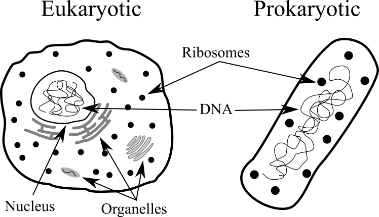
Figure 1:The main differences and similarities between eukaryotic and prokaryotic cells. The cells have not been drawn at scale.
- Cell
- A cell is the basic structural and functional unit of all living organisms. It is the smallest unit capable of carrying out the processes necessary for life, such as energy production, metabolism, and reproduction.
- Organelles
- Specialized structures within cells that perform distinct functions necessary for cellular life. Organelles make it possible to carry out tasks in isolation from the rest of the cell, ensure that the cell operates efficiently and responds to its environment.
- Procaryotes
- Unicellular organisms that lack a true nucleus and membrane-bound organelles. Their genetic material is located in a nucleoid, and they typically have a single, circular chromosome along with plasmids. Prokaryotic cells have a rather small size () and reproduce through binary fission[4]. Most have a rigid cell wall made of peptidoglycan (in bacteria). Examples of prokaryotes include bacteria and archaea.
- Eukaryotes
- Organisms whose cells contain a true nucleus enclosed by a nuclear membrane and various membrane-bound organelles such as mitochondria, endoplasmic reticulum, and Golgi apparatus. Their DNA is linear and organized into chromosomes within the nucleus. Eukaryotic cells are generally larger than prokaryotes () and reproduce through mitosis for somatic cells and meiosis for gametes. While some eukaryotes have cell walls (e.g., plants and fungi), others do not. Examples of eukaryotes include plants, animals, fungi, and protists.
3.2Macromolecules and polymers
A macromolecule is a molecule composed by a great number of covalently bonded atoms[5]. The most common class of macromolecules is that of polymers, which are molecules composed by smaller subunits, the monomers, covalently linked together. If the monomers are all of the same type, the resulting molecule is a homopolymer, while if they are different, the molecule is a heteropolymer. In general, monomers can be connected in different ways, giving raise to unidimensional structures such as chains or rings, or to more complicated topologies such as brushes, stars, networks, etc.
Focussing on chains, the number of repeating units (also known as residues) composing a polymer is called degree of polymerisation , and for common plastic materials is rather large (). The simplest polymer is the hydrocarbon polyethylene, , which is used to make cheap bags and bottles and accounts for more than of the plastic produced worldwide (see e.g. Geyer et al. (2017)). Other very common polymers used to build everyday objects are polypropilene, , which is heat- and fatigue-resistant and therefore used to make hinges, piping systems, containers, and polystyrene, , used to make plastic cutlery, containers or insulating foams. The skeletal formulas of these three polymers are shown in Figure 2.
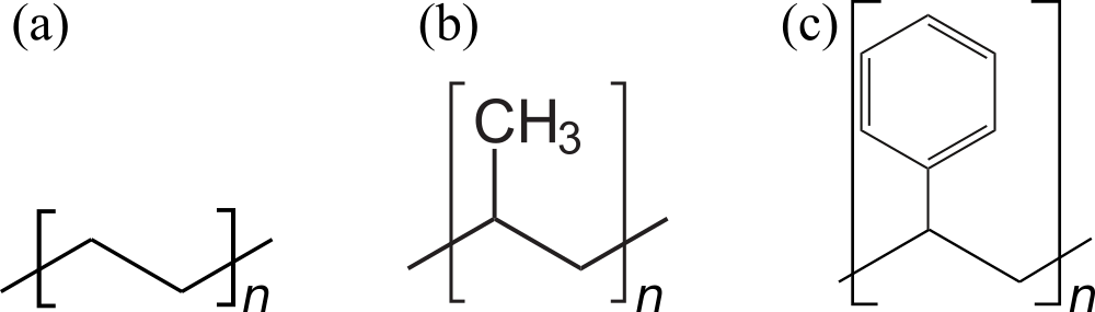
Figure 2:The skeletal formulas of (a) polyethylene, (b) polypropilene and (c) polystyrene. Here the repeating unit in (a) is to make it more easy to compare it with the other two.
In the biological context, three of the four main macromolecular components of life are polymers: proteins, nucleic acids and carbohydrates, also known as biopolymers. While there exist (bio)polymeric substances with more complex architectures, the main macromolecules of life have a linear (chain) structure that makes it possible to assign a one dimensional sequence to each molecule. This sequence is just the list of monomers composing the chain, spelt from one chain end to the other.
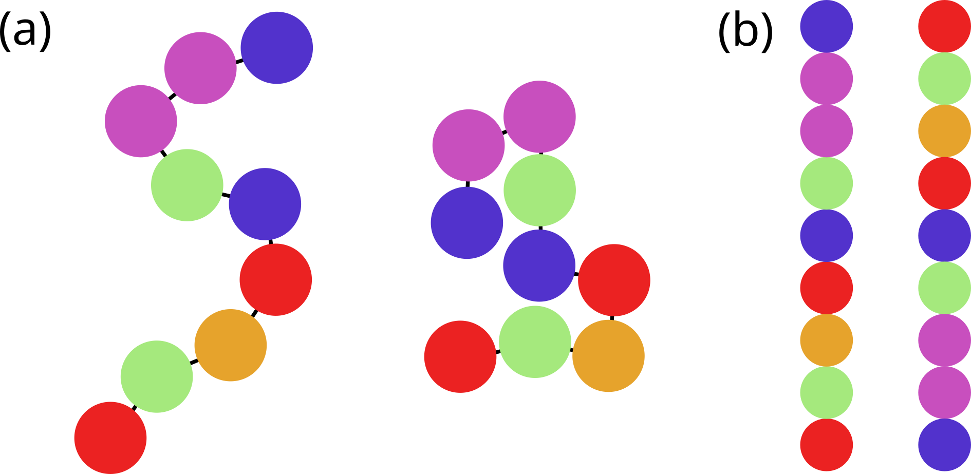
Figure 3:A cartoon of a polymer composed by 9 monomers (the coloured spheres) connected by covalent bonds (black lines). Panel (A) shows two 2D conformations, panel (B) shows the two 1D sequences built by listing the monomers that make up the chain, starting from either end.
Figure 3 shows an imaginary short polymer composed by 9 monomers of different nature (coloured differently). In general, there are many different spatial arrangements that the same (bio)polymer can take in solution. By contrast, its sequence is fixed, being given by the list of covalently-linked monomers. However, as shown in the figure, in absence of any convention, the sequence can be read from either end, giving raise to an ambiguity. As we will see, there exist conventions for proteins and nucleic acids that get rid of this ambiguity.
3.2.1Some useful observables
First, some definitions.
- End-to-end vector,
- The vector distance between the first and last residue of a polymer chain. Its length is the end-to-end distance, .
- Contour length,
- The maximum possible end-to-end distance, which is achieved for a fully-extended polymer chain.
- Monomer position,
- The position of the -th monomer.
- Bond vector,
- The vector connecting the and -th residues, defined as .
- Chemical distance
- The number of bonds separating two monomers along the chain, i.e. for monomers and .
- Ideal chain
- A chain in which two residues that are far from each other, i.e. residues and for which , do not interact.
Consider a polymer chain composed by monomers connected by bonds. Its instantaneous end-to-end vector is
Consider the ensemble average of this quantity, , which denotes an average over all possible states of the system (accessed either by considering many chains or many different conformations of the same chain). In this particular case the ensemble average corresponds to averaging over an ensemble of chains having bonds, with all possible bond orientations. Since there is no preferred direction in this ensemble, the average end-to-end vector is zero[6]. A simple non-zero average that can be built out of the end-to-end vector is
If the bond vectors are all of the same length (which is often a good approximation, given the rigidity of the backbone covalent bonds), , where is the angle between and , and the mean-squared end-to-end distance can be written as
Note that in this case the contour length has the simple expression .
In the simplest polymer model there is no correlation between any two monomers and . In such a freely-jointed chain the average cosine vanishes if , since
and therefore the double sum in Eq. (3) becomes a single sum of ones, yielding
However, in a typical ideal chain, only if and are sufficiently far apart from each other. In this case, if we assume that there is a maximum chemical distance beyond which , we can write the inner sum of Eq. (3) as
where [7], the so-called Flory’s characteristic ratio, accounts for the local monomer-monomer correlations due to steric hindrances and hampered rotations around chemical bonds and varies from polymer to polymer. For these ideal chains, Eq. (3) can be written as
Flexible polymers have many universal properties that are independent of the local chemical structure, and they can all be described in terms of equivalent freely-jointed chains. The equivalent chain has the same mean-squared end-to-end distance and contour length, but a different number of effective beads of length , chosen to match the values of and :
so that
The effective bond length is known as Kuhn’s length, and it represents the size of a segment that behaves as a freely-jointed monomer in the equivalent chain.
The size of a linear chain is well-described by the square root of its mean-squared end-to-end distance, . However, in some cases this quantity is not well defined (e.g. for ring or branched polymers), or it is not easily accessible in experiments. In these cases it is useful to define the radius of gyration, which can be computed for any set of atoms or particles:
where is the position of the centre of mass of the polymer. Sometimes (also in simulations), it is not convenient, or possible, to compute the centre of mass. For these cases, Eq. (10) can be rewritten in another form by substituting the definition of , obtaining
where we have first completed the square of the binomial by duplicating the double sum (hence the factor of 2 at the denominator), and then run the inner sum on monomers having index , so that each pair of monomers only enters once in the double sum. The associated ensemble average is then
The radius of gyration and end-to-end distance are closely related. For instance, for a freely-jointed chain, it can be demonstrated that
which means that the two quantities scale with in the same way. This proportionality holds also for other (more complicated) models.
In general, for large enough degrees of polymerisation (i.e. for ), polymers are scale-free objects, which means that most of their properties can be expressed as power laws in . A special role is played by the exponent that connects to the polymer size (i.e. its gyration radius or end-to-end distance), which is called :
where for an ideal chain. Self-avoiding polymers, i.e. polymers whose only interaction is repulsive, have , which means that they are swollen with respect to ideal polymers: their linear size is larger than it would be if there was no repulsion. Compare it with the scaling of the linear size of a dense object, for which .
3.3DNA
Deoxyribonucleic acid (DNA) is a macromolecule that stores the genetic information of an organism. DNA contains regions called genes, which encode for proteins to be produced. Other regions of the DNA contain regulatory elements, which partially influence the level of expression of each gene. Within the genetic code of DNA lies both the data about the proteins that need to be encoded, and the control circuitry, in the form of regulatory motifs.
As we will see in depth, in cells DNA is usually found in a “double-stranded” helical form, where each strand is a long chain of repeating units, called nucleotides, of just four types: A(adenine), C(cytosine), T (thymine), and G (guanine). The list of nucleotides is called sequence or primary structure. In the double strand, A pairs with T and G with C, with the A-T pairing being weaker than the C-G pairing[8].
The two DNA strands in the double helix are complementary, meaning that if there is an A on one strand, it will be bonded to a T on the other, and if there is a C on one strand, it will be bonded to a G on the other. The DNA strands have a chemical directionality, or polarity, with the convention being to list a strand’s sequence with the direction along which enzymes[9] called polymerases[10] synthesise DNA and RNA, called the 5’ to 3’ direction. With this in mind, we can say that that the DNA strands are anti-parallel, as the 5’ end of one strand is adjacent to the 3’ end of the other. As a result, DNA can be read both in the 3’ to 5’ direction and the 5’ to 3’ direction, and genes and other functional elements can be found in each.

Figure 4:The multi-scale organisation of DNA in a eukaryotic cell. Adapted from a figure made by Phrood, via Wikimedia Commons.
Base pairing between nucleotides of DNA constitutes its secondary structure. In addition to DNA’s secondary structure, there are several extra levels of structure that allow biological DNA to be tightly compacted and influence gene expression, as schematically shown in Figure 4. The tertiary structure describes the twist in the DNA ladder that forms a helical shape. In the quaternary structure, DNA is tightly wound around small proteins called histones. These DNA-histone complexes are further wound into tighter structures seen in chromatin.
Before DNA can be replicated or transcribed into RNA, the chromatin structure must be locally “unpacked”. Thus, gene expression may be regulated by modifications to the chromatin structure, which make it easier or harder for the DNA to be unpacked. This regulation of gene expression via chromatin modification is an example of epigenetics.
The structure of DNA allows the strands to be easily separated for the purpose of DNA replication, as well as transcription, translation, recombination, and DNA repair, among others. This was noted by Watson and Crick as “It has not escaped our notice that the specific pairing that we have postulated immediately suggests a possible copying mechanism for the genetic material”. In the replication of DNA, the two complementary strands are separated, and each of the strands are used as templates for the construction of a new strand.
DNA polymerases attach to each of the strands at the origin of replication, reading each existing strand from the 3’ to 5’ direction and placing down complementary bases such that the new strand grows in the 5’ to 3’ direction. Because polymerases build the chains from 5’ to 3’, one strand (the leading strand) can be copied continuously, while the other (the lagging strand) grows in pieces which are later glued together by another enzyme, DNA ligase. The end result is 2 double-stranded pieces of DNA, where each is composed of one old strand, and one new strand; for this reason, DNA replication is a semiconservative process.
Many organisms have their DNA split into several chromosomes. Each chromosome contains two strands of DNA, which are complementary to each other but are read in opposite directions. Genes can occur on either strand of DNA. The DNA before a gene (in the 5’ region) is considered “upstream”, whereas the DNA after a gene (in the 3’ region) is considered “downstream”. Figure 5 shows the genome size ranges of various forms of life.
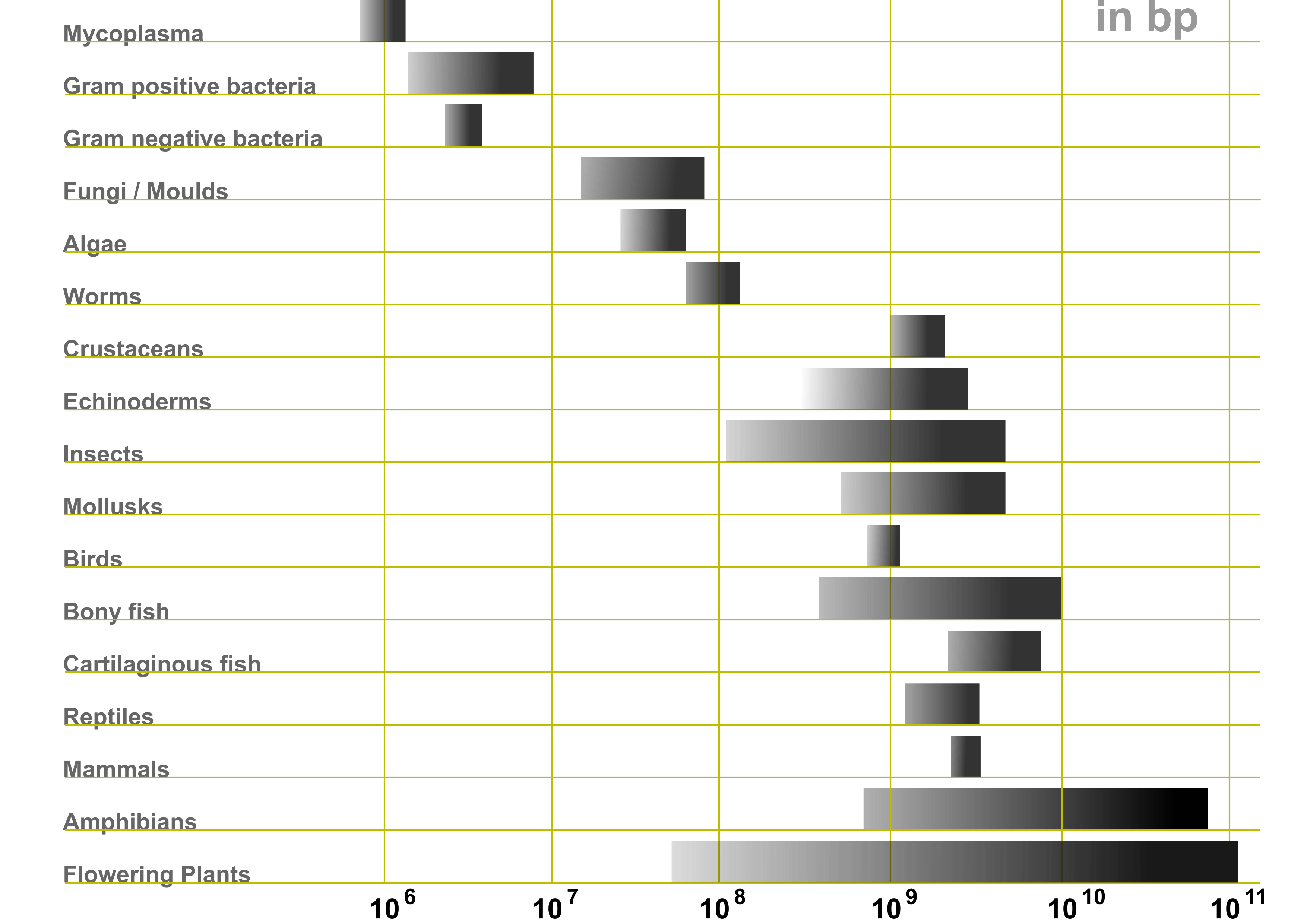
Figure 5:Genome size ranges (in base pairs) of various life forms. Credits to Abizar via Wikipedia Commons.
3.4Transcription and RNA

Figure 6:A sketch showing three steps that lead to the synthesis of an mRNA: RNA polymerase (RNAp) attaches to the transcription start site (transcription initiation) and start building an RNA chain that is fully complementary to the DNA template strand (transcription elongation). When the gene has been fully transcribed, the RNAp and mRNA both detach and leave (transcription termination). Adapted from here, here, and here.
When a gene product is to be expressed, the associated DNA is partially unwound to form a “bubble”, where the two strands are separated. At this point transcription, which is the process by which RNA is produced using a DNA template, can commence: RNA polymerase is recruited to the transcription start site by regulatory protein complexes, and then reads the DNA from the 3’ to 5’ direction, placing down complementary bases to form a messenger RNA (mRNA) strand[11]. RNA uses the same nucleotides as DNA, except Uracil is used instead of Thymine.
mRNA in eukaryotes experience post-translational modifications, or processes that edit the mRNA strand further, starting from the “pre-mRNA” molecule that is complementary to the template DNA strand of a gene. Most notably, a process called splicing removes introns, regions of the gene which don’t code for protein, so that only the coding regions, the exons, remain. Different regions of the primary transcript may be spliced out to lead to different protein products (alternative splicing). In this way, an enormous number of different molecules may be generated based on different splicing permutations. In addition to splicing, both ends of the mRNA molecule are processed. The 5’ end is capped with a modified guanine nucleotide, while at the 3’ end, roughly 250 adenine residues are added to form a poly(A) tail. In most cases, the final molecule will be used by the cell machinery (and, in particular, by ribosomes) to synthesise proteins. As we will see in a moment, the base unit of a protein is an amino acid, and the information about what amino acid to add to the nascent protein is stored in the mRNA as a three-nucleotide sequence, also known as a codon.
RNA is not only the intermediary step to code a protein, but RNA molecules also have catalytic and regulatory functions. Though proteins are generally thought to carry out the main cellular functions, it has been shown that RNA molecules can have complex three-dimensional structures and perform diverse functions in the cell. In 1989 the Chemistry Nobel Prize was awarded to Thomas R. Cech and Sidney Altman for their “discovery of catalytic properties of RNA”, which greatly contributed to the establishment of the concept of ribozymes (ribonucleic acid enzymes), which are RNA molecules that have the ability to catalyze specific biochemical reactions.
The most common RNA types are:
mRNA (messenger RNA) contains the information to make a protein and is translated into protein sequence.
tRNA (transfer RNA) specifies codon-to-amino-acid translation. It contains a 3 base pair anti-codon complementary to a codon on the mRNA, and carries the amino acid corresponding to its anticodon attached to its 3’ end.
rRNA (ribosomal RBA) forms the core of the ribosome, the organelle responsible for the translation of mRNA to protein.
snRNA (small nuclear RNA) is involved in splicing (removing introns from) pre-mRNA, as well as other functions.
The discovery of rybozymes contributed to the “RNA world” hypothesis, for which early life was based entirely on RNA. RNA served as both the information repository (like DNA today) and the functional workhorse (like protein today) in early organisms. Protein is thought to have arisen afterwards via ribosomes, and DNA is thought to have arisen last, via reverse transcription.
3.5Translation and the genetic code
Translation is the process by which the information encoded in mRNA is used to synthesize a protein. Unlike transcription, where the nucleotide sequence in DNA is transcribed into a corresponding nucleotide sequence in RNA, translation involves converting this nucleotide sequence into an amino acid sequence, forming the primary structure of the protein. Since there are 20 different amino acids and only 4 nucleotides, the mRNA is read in sets of three nucleotides, known as codons, each of which specifies a particular amino acid.

Figure 7:The meaning of each sequence made of three nucleotides (also known as a codon or codon triplet), as read by the ribosome. Each codon should be spelt starting from the inner circle and going outwards. The outer circle shows what corresponds to each codon.
Figure 7 shows the meaning of each codon. Since each nucleotide in a codon can have one out of 4 possible values (A, C, G or T), there exist possible codons. Out of these 64 combinations, three are recognised as “stop signals”, while the rest encode amino acids, with the exception of the AUG codon which, in addition to represent methionine, is also typically used to initiate protein syntesis. Since there are 64 possible codon sequences, the code is degenerate, and most amino acids (excluding methionine and tryptophan) are encoded by more than a single codon. Most of the degeneracy occurs in the 3rd codon position.
The outer circle of Figure 7 contains the list of standard amino acids, together with their three- and one-letter abbreviations, which are shown in bold and after each AA name, respectively.
3.6Information flow: the central dogma of biology
The single most important fact about biology is the so-called “central dogma of biology”, which is a framework that describes the flow of genetic information in biological systems. It was formulated by Francis Crick[12] and presented to the public in a famous lecture given on September 19th in 1957 Cobb (2017). The first formulation of the central dogma is shown in Figure 8, where arrows indicate the flow of information: what is used to build what. Note that DNA protein and RNA DNA information transfers were highly speculative at that time (and in fact DNA protein transfers have not been observed in vivo).
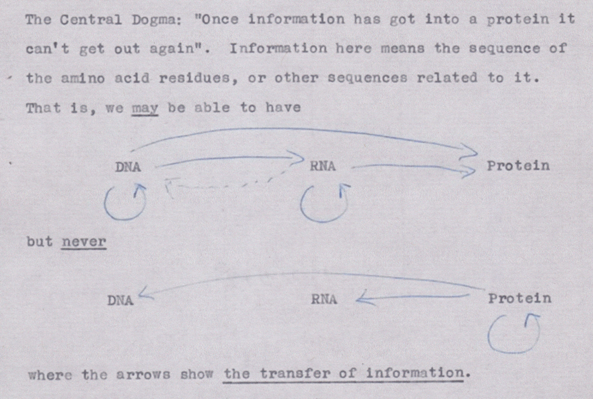
Figure 8:The first outline of the central dogma, from un unpublished note made by Crick in 1956. Credits: Wellcome Library, London. Taken from Cobb (2017).
In later formulations Crick expanded and clarified his view on this matter, writing that
the central dogma could be stated in the form “once (sequential) information has passed into protein it cannot get out again”.
[...]
the central dogma was a negative statement, saying that transfers from protein did not exist.
Nota Bene: this version of the central dogma is not only the original one, but also the only one that stood the test of time: popularised versions such as “DNA RNA protein” or “DNA makes RNA, RNA makes protein” are oversimplified and ambiguous statements[13].
3.7The experimental characterisation of the structure of biomolecules
I will refer to this part when talking about the secondary and tertiary structure of proteins and nucleic acids.
3.7.1Secondary structure
Several experimental methods can be used to understand the secondary structure of a particular biomolecule, such as proteins or nucleic acids. Here are some common techniques:
Circular Dichroism (CD) Spectroscopy: CD spectroscopy is widely used to study the secondary structure of proteins. It measures the difference in the absorption of left-handed versus right-handed circularly polarized light, providing information about the overall content of -helices, -sheets, nucleic acid helices, and random coils.
Fourier Transform Infrared (FTIR) Spectroscopy: FTIR spectroscopy measures the absorption of infrared light by the biomolecule, which provides information about the types of chemical bonds and functional groups present. The amide I and II bands are particularly informative for analyzing protein secondary structures.
Ultraviolet (UV) Absorption Spectroscopy: UV absorption spectroscopy can provide some information about the secondary structure, especially in nucleic acids. It is less informative for proteins compared to CD spectroscopy but can still be useful when combined with other techniques.
3.7.2Three-dimensional structure
The 3D structure of biomacromolecules such as proteins and nucleic acids can be experimentally determined using several techniques. The most commonly used methods are:
X-ray Crystallography:
Procedure: The biomolecule is crystallized, and then X-rays are directed at the crystal. The X-rays diffract as they pass through the crystal, creating a diffraction pattern that can be recorded. The diffraction pattern is analyzed to determine the electron density map, which is used to model the atomic structure of the biomolecule.
Advantages: High resolution, can be used for large biomolecules.
Limitations: Requires high-quality crystals, which can be difficult to obtain for some biomolecules (e.g. molecules that are not soluble in water, like many membrane proteins).
Nuclear Magnetic Resonance (NMR) Spectroscopy:
Procedure: The biomolecule is dissolved in solution, and NMR spectra are obtained by applying a magnetic field and measuring the resulting interactions between nuclear spins. The spectra provide information about the distances and angles between atoms, which are used to calculate the 3D structure.
Advantages: Provides information about the dynamics and flexibility of biomolecules in solution.
Limitations: Generally limited to smaller biomolecules (up to about 50 kDa, i.e. amino acids or nucleotides), although recent advances are pushing these limits.
Cryo-Electron Microscopy (cryo-EM):
Procedure: The biomolecule is rapidly frozen in a thin layer of ice, and then imaged using an electron microscope. Thousands of 2D images are collected and computationally combined to reconstruct a 3D model of the biomolecule.
Advantages: Does not require crystallization, suitable for large and complex biomolecules, including those that are difficult to crystallize.
Limitations: Typically lower resolution than X-ray crystallography, although recent advances have significantly improved the resolution.
Small-Angle X-ray Scattering (SAXS):
Procedure: The biomolecule is dissolved in solution, and X-rays are scattered at small angles by the sample. The scattering pattern provides low-resolution information about the overall shape and size of the biomolecule.
Advantages: Can study biomolecules in near-physiological conditions, provides information about conformational changes and flexibility.
Limitations: Lower resolution compared to X-ray crystallography and cryo-EM, providing only general shape information.
3.8Some useful numbers and quantities
| Quantity | Value |
|---|---|
| at 298 K | J |
| " | |
| RT at 298 K | |
| " | |
| Average nucleotide mass | Da |
| Average amino acid mass | Da |
4Introduction to computational physics
Computational physics is a branch of physics that utilizes computational methods and numerical analysis to solve physical problems that are difficult or impossible to solve analytically. It involves the development and application of algorithms, numerical techniques, and computer software to simulate physical systems, analyze experimental data, and predict the behavior of natural phenomena.
At its core, computational physics merges principles from theoretical physics, applied mathematics, and computer science. It covers a wide range of topics, including classical mechanics, quantum mechanics, statistical mechanics, electrodynamics, condensed matter physics, biophysics, and more. In these days, high-performance computing is often required to perform large-scale simulations and calculations, which are essential for understanding physical processes where many length- and time-scales are involved, which happens often in various domains such as astrophysics, material science, biophysics, and climate modeling.
The methods employed in computational physics vary greatly, and include solving (partial) differential equations, performing molecular simulations, and employing finite element analysis. These techniques allow physicists to model systems at different scales, from subatomic particles to cosmological structures. Interestingly, many of the methods can be applied in multiple fields.
Another important field of application of computational physics is the interpretation of experimental data. By simulating experiments and comparing the results with actual measurements, computational physicists can refine theoretical models and improve the accuracy of predictions. This iterative process enhances our understanding of the underlying physical principles, and can help to uncover new phenomena.
Despite the enormous variety of methods and applications, there are some common concepts that are essential for anyone venturing in the subject, regardless of the specific subfield they choose. Some of these are technical, and are listed in the prerequisite section. Here, I will highlight two additional skill sets that every aspiring computational physicist should develop:
Bridging Theory and Experiment: Historically known as “computer experiments”, computer simulations sit in the middle between theory and experiment. A proficient computational physicist can effectively bridge these two realms, provided he develops a familiarity with the specific jargon, techniques, and methodologies of both fields. This dual expertise is a significant advantage. However, it is sometimes hard to find a fit in a dichotomic world, where “theory or experiment” is all there is. Fortunately, that world is dying (but has not died yet).
Algorithmic Problem Solving: Problem-solving is a critical skill for any physicist, often involving the application of algorithmic reasoning to find solutions. For computational physicists, the ability to think in terms of algorithms is even more crucial. Developing this skill enables them to tackle complex problems systematically and effectively. During the course I will present many algorithms used to tackle some specific (bio)physical problems. Most of the time there will be an accompanying pseudo-code or real code, but in some cases you will be asked to do it yourself.
To get thing started, I will present a programming technique that will be applied later to some biophysical problems. However, before doing that, let’s brush up our Python skills with this notebook.
4.1Dynamic programming
At the most simple level, the three groups of biomolecules introduced above (DNA, RNA, and proteins) can be described in terms of a primary structure, which is just a sequence of characters. These characters are taken from a set called alphabet. DNA and RNA have alphabets of four characters (A, C, G, and T or U), while the protein alphabet is composed of 20 elements (the 20 amino acids). While the properties of any of these molecules are determined by their 3D structure, the latter depends, often in a very complicated manner, on their sequence. Therefore, it is most useful to develop tools and methods that can work efficiently with (possibly very long) 1D sequences.
For this reason, I will introduce dynamic programming, which is an algorithmic technique that shines at solving optimisation problems on sequences and trees. The main idea is to write the solution of a given complex problem in terms of simpler subproblems that can be solved. The solution to the original problem can then be “traced back” from the solutions of the simpler problems. A typical dynamic programming algorithm has two phases:
The fill-in phase, in which a so-called dynamic programming matrix (or table) is filled in. The dynamic programming matrix contains the scores of the subproblems, and once it has been filled, only the score of the solution is known, and not the solution itself.
The trace-back phase, in which the matrix is traversed back from the optimal score to the beginning to obtain the optimal solution (or solutions).
I will apply dynamical programming to the “coin change” toy problem. We will see later on how to apply it to more biologically relevant contexts.
4.1.1The coin change problem
There are several variations to this problem. We start with the following: given an amount of money and a set of types of coins, what is the minimum number of coins that can change ? Here is an example: for and , the minimum number of coins is 3, since .
The simplest way of solving the problem is by enumerating all possible ways can be changed with the coins in , and then picking the one containing the fewest amount of coins. However, this algorithm performs worse and worse as and increases. Can we estimate by how much?
Using the notation introduced in the box, we can estimate the cost of the “brute-force” algorithm as follows. Given an amount and a coin , a solution can either not contain , or contain it up to times. As a result, we have ways of using each coin , and we have such coins. Disregarding multiplying constants and lower-order terms, the overal complexity is then . It is hard to overstate how bad is such a scaling. We have to do better!
Let’s try with a “greedy” algorithm: we find a solution by taking the largest coin that is smaller than and applying the same operation to , until the remaining amount becomes zero. Applying this algorithm to the example above would immediately yield the correct solution. The algorithmic complexity is also much better: the worst-case scenario is the one where we use coins of the same size, which would yield . However, the algorithm requires that at each iteration we find the largest coin that is smaller than the residual amount. This can be done by either looping over at each iteration, which would make the complexity , or, which is much better, by sorting beforehand, so that the total algorithmic complexity would be . This is much better than an exponential complexity. Unfortunately, greedy algorithms are known to be heavily attracted to local minima. For instance, if and , the greedy algorithm would yield a solution with 4 coins, since . However it is clear that the best solution in this case is .
We need an algorithm that is fast but does reliably find the correct solution. In order to do so, we need to find a way of casting the solution to the problem in terms of solutions of subproblems. To do so we define the accessory function :
where is the minimum number of coins necessary to change . We now make the crucial observation that
Eq. (16), for which I will provide a proof, shows that the best way to make change for depends on the best way to make change for smaller amounts.
We can now leverage Eq. (16) to calculate the minimum number of coins necessary to change any amount with a time that is linear in and in the number of coin types, , i.e. with an algorithmic (time) complexity . First, we apply Eq. (16) to progressively build a table containing the values, with , starting from :
DEFINE C as the set of possible coins
DEFINE N as the amount we want to change
DEFINE table as an array with N + 1 entries
DEFINE function w(x)

table[0] = 0
FOR each value x between 1 and N
   SET table[x] to the mininum value of {w(x - c) + 1}, where c is any coin in C
Program 1:Pseudocode for the fill-in phase.
Once the table is ready, the answer to our question about the minimum number of coins can be read off its last entry, . However, if we want to know the details of the solution, e.g. which coins add up to , we have to trace back Eq. (16):
ASSUME the definitions of the fill-in block
SET x = N
DEFINE S as an empty list

WHILE x is larger than 0
   FIND a coin c in C for which table[x] = table[x - c] + 1
   ADD c to S
   SET x to x - c
Program 2:Pseudocode for the trace-back phase.
You can find a Python implementation of the brute-force and dynamic-programming algorithms here. Note that two brute-force version returns only the optimal number of coins and not the solution itself. Here is a list of things you can do with this code to brush up your coding and plotting skills:
Easy: Port the code to another programming language you know (e.g. C).
Medium: Use this code or yours to “experimentally” find out the algorithmic complexity of the two codes, in terms of and . In order to do so, solve the coin change problem for a bunch of combinations[14], measure the time it takes the code to find the optimal solution, and plot the two sets of results ( and ).
Hard: Extend the brute-force solution so that it also returns an optimal solution.
Hard: Extend the dynamic-programming solution so that it returns all optimal solutions.
like this.
Or at least it does not come with a Unix-like (POSIX) terminal, which is what we will be using.
Penalties will be given if I realise a student does not understand what they did, or why, during the oral exam.
For what concerns us, this is a simpler version of mitosis.
“great number” is a purposedly vague qualifier: there is no strict definition about the number of atoms required for a molecule to be dubbed a macromolecule.
You can find the same result by realising that an ideal polymer is just a random walk of steps: if the random walk is not biased, the probability of moving towards a direction is independent of the directions taken before, and therefore, on average, the walker does not move.
It is larger than one since , and the terms are all positive.
For this reason, the genetic composition of bacteria that live in hot springs is G-C.
Since the template strand is read 3’ 5’, the nascent mRNA is built in the 5’ 3’ direction.
Apparently Crick was not familiar with the meaning of “dogma”, which is why he used that word instead of other options that would have perhaps avoided later misunderstandings (see e.g. Cobb (2017)).
Oversimplified because they leave out important information transfers such as RNA RNA and RNA DNA, but also ambiguous since the meaning of arrows and “makes” are not spelt out.
in some cases it may be worth averaging over different at fixed .
- Lehninger, A. L., Nelson, D. L., & Cox, M. M. (2005). Lehninger principles of biochemistry. Macmillan.
- Finkelstein, A. V., & Ptitsyn, O. (2016). Protein physics: a course of lectures. Elsevier.
- Leach, A. R. (2001). Molecular modelling: principles and applications. Pearson education.
- Schlick, T. (2010). Molecular modeling and simulation: an interdisciplinary guide (Vol. 2). Springer.
- Frenkel, D., & Smit, B. (2023). Understanding molecular simulation: from algorithms to applications. Elsevier.
- Israelachvili, J. N. (2011). Intermolecular and surface forces. Academic press.
- Giustino, F. (2014). Materials modelling using density functional theory: properties and predictions. Oxford University Press.
- Böttcher, L., & Herrmann, H. J. (2021). Computational Statistical Physics. Cambridge University Press.
- Anderson, P. W. (1972). More Is Different: Broken symmetry and the nature of the hierarchical structure of science. Science, 177(4047), 393–396. 10.1126/science.177.4047.393
- Geyer, R., Jambeck, J. R., & Law, K. L. (2017). Production, use, and fate of all plastics ever made. Science Advances, 3(7). 10.1126/sciadv.1700782
- Rubinstein, M., & Colby, R. H. (2003). Polymer physics. Oxford university press.
- WATSON, J. D., & CRICK, F. H. C. (1953). Molecular Structure of Nucleic Acids: A Structure for Deoxyribose Nucleic Acid. Nature, 171(4356), 737–738. 10.1038/171737a0
- Cobb, M. (2017). 60 years ago, Francis Crick changed the logic of biology. PLOS Biology, 15(9), e2003243. 10.1371/journal.pbio.2003243
- CRICK, F. (1970). Central Dogma of Molecular Biology. Nature, 227(5258), 561–563. 10.1038/227561a0