Crash course on Python

Based on this notebook by Rick Muller, licensed under a Creative Commons Attribution-ShareAlike 3.0 Unported License.

Note that the original notebook is much longer and detailed.

1Python Overview¶

This is a quick introduction to Python. There are lots of other places to learn the language more thoroughly. I have collected a list of useful links, including ones to other learning resources, at the end of this notebook. If you want a little more depth, Python Tutorial is a great place to start, as is Zed Shaw’s Learn Python the Hard Way.

The lessons that follow make use of Jupyter notebooks. Briefly, notebooks have code cells (that are generally followed by result cells) and text cells. The text cells are the stuff that you’re reading now.

1.1What You Need to Install¶

These notes assume you have a Python distribution that includes:

• Python;
• Numpy, the core numerical extensions for linear algebra and multidimensional arrays;
• Scipy, additional libraries for scientific programming;
• Matplotlib, excellent plotting and graphing libraries;
• Jupyter, with the additional libraries required for the notebook interface.

The easiest way to install and update all of these is using the Anaconda package, which contains everything you need for scientific programming.

1.2Using Python as a Calculator¶

Many of the things I used to use a calculator for, I now use Python for:

Differently from C, in Python an integer division does what you would expect:

However, sometimes it can be useful to do a proper truncating divisions. In these cases you can use the // operator:

Python libraries are called modules, and can be imported with an import statement. As an example, consider the math module, which is a standard module containing many useful mathematical functions and constants. We can either import the whole module or just the thing(s) we need:

You can define variables using the equals (=) sign:

If you try to access a variable that you haven’t yet defined, you get an error:

You can name a variable almost anything you want. It needs to start with an alphabetical character or “_”, can contain alphanumeric charcters plus underscores (“_”). Certain words, however, are reserved for the language:

and, as, assert, break, class, continue, def, del, elif, else, except,
exec, finally, for, from, global, if, import, in, is, lambda, not, or,
pass, print, raise, return, try, while, with, yield

Trying to define a variable using one of these will result in a syntax error:

The Python Tutorial has more on using Python as an interactive shell.

1.3Strings¶

Strings are lists of printable characters, and can be defined using either single quotes

or double quotes

But not both at the same time, unless you want one of the symbols to be part of the string.

Just like the other two data objects we’re familiar with (integer and floating numbers), you can assign a string to a variable

The print statement is often used for printing character strings:

The print function can also print data types other than strings:

In the above snippet, the number 600 (stored in the variable “area”) is converted into a string before being printed out.

You can use the + operator to concatenate strings together:

Don’t forget the space between the strings, if you want one there.

You can use + to concatenate multiple strings in a single statement:

or use commas:

If you have a lot of words to concatenate together, there are other, more efficient ways to do this. But this is fine for linking a few strings together.

1.4Lists¶

Very often in a programming language, one wants to keep a group of similar items together. Python does this using a data type called lists.

You can access members of the list using the index of that item:

As in C, the index of the first element of a list is 0. Thus, in this example, the 0 element is “Sunday”, 1 is “Monday”, and so on.

Differently from C, If you need to access the n-th element from the end of the list, you can use a negative index. For example, the -1 element of a list is the last element:

You can add additional items to the list using the .append() method:

The range() command is a convenient way to make sequences of numbers:

To see the items in the range, you can make a list of it.

Note that range(n) starts at 0 and gives the sequential list of integers less than n. If you want to start at a different number, use range(start, stop)

The lists created above with range have a step of 1 between elements. You can also give a fixed step size via a third command:

Lists do not have to hold the same data type. For example,

You can find out how long a list is using the len() command:

1.5Iteration, Indentation, and Blocks¶

One of the most useful things you can do with lists is to iterate through them, i.e. to go through each element one at a time. To do this in Python, we use the for statement:

(Almost) every programming language defines blocks of code in some way. In C, one uses curly braces {} to define these blocks.

Python uses a colon, :, followed by indentation level to define code blocks. A block is made by consecutive lines that have the same indentation level. In the above example the block was only a single line, but we could have had longer blocks as well:

The range() command is particularly useful with the for statement to execute loops of a specified length:

1.6Slicing¶

Strings are sequences of things, just like lists. Therefore, as with lists, you can iterate through the letters in a string:

This is only occasionally useful. Slightly more useful is the slicing operation, which you can also use on any sequence. We already know that we can use indexing to get the first element of a list:

By extending this notation, we can obtain subsequences. For instance, a sequence containing the first two elements of a list can be generated with

or simply

If we want the last items of the list, we can do this with negative slicing:

which is somewhat logically consistent with negative indices accessing the last elements of the list.

You can do:

The same technique can be applied to strings:

If we really want to get fancy, we can pass a third element into the slice, which specifies a step length (just like a third argument to the range() function specifies the step):

Note that in this example the second argument was omitted, so that the slice started at 2, went to the end of the list, and took every second element, to generate the list of even numbers less that 40.

1.7Booleans and Truth Testing¶

Contrary to C, Python has builtin boolean variables, i.e. that can be either True or False, and can be used with if statements:

(note that the day variable was set in a previous cell). In Python, conditional expressions are also booleans. For instance:

As in C, the == operator performs equality testing. If the two items are equal, it returns True, otherwise it returns False. In this case, it is comparing two variables, the string "Sunday", and whatever is stored in the variable day, which, in this case, is the other string "Saturday". Since the two strings are not equal to each other, the truth test has the false value.

The if statement that contains the truth test is followed by a code block (a colon followed by an indented block of code). If the boolean is true, it executes the code in that block. Since it is false in the above example, we don’t see that code executed.

The first block of code is followed by an else statement, which is executed if nothing else in the above if statement is true. Since the value was false, this code is executed, which is why we see “Go to work”.

You can compare any data types in Python:

We see a few other boolean operators here, all of which which should be self-explanatory. Less than, equality, non-equality, and so on.

Particularly interesting is the 1 == 1.0 test, which is true, since even though the two objects are different data types (integer and floating point number), they have the same value.

We can do boolean tests on lists as well, although the behaviour is somehow counterintuitive: for equality, it works as you would expect, and the comparison is carried out element-wise:

For inequalities, the comparison is still done element-wise, although the comparison result is determined by the comparison of the first unequal elements. Any other subsequent element does not affect the result.

Finally, note that you can also string multiple comparisons together, which can result in very intuitive tests:

If statements can have elif parts (which is a contraction of “else if”), in addition to if/else blocks. For example:

Note that ordinary data types have boolean values associated with them. Indeed, casting anything that has a 0 value (the integer or floating point 0, an empty string "", or an empty list []) to a boolean will return False:

1.8Code Example: The Fibonacci Sequence¶

The Fibonacci sequence is a sequence in math that starts with 0 and 1, and then each successive entry is the sum of the previous two. Thus, the sequence goes 0, 1, 1, 2, 3, 5, 8, 13, 21, 34, 55, 89, ...

A very common exercise in programming books is to compute the Fibonacci sequence up to some number n.

Note that in Python # starts a comment.

1.9Functions¶

We might want to use the Fibonacci snippet with different sequence lengths. We could cut and paste the code into another cell, changing the value of n, but it’s easier and more useful to make a function out of the previous snippet code:

We can now call fibonacci() for different sequence_lengths:

We’ve introduced a several new features here. First, note that the function itself is defined as a code block (a colon followed by an indented block). This is the standard way that Python delimits things. Next, note that the first line of the function is a single string. This is called a docstring, and is a special kind of comment that is often available to people using the function through the python command line:

If you define a docstring for all of your functions, it makes it easier for other people to use them, since they can get help on the arguments and return values of the function.

Note that I have also added some ifs to handle corner cases, and possibly issue a warning if the given length is not right.

1.10Recursion and Factorials¶

Functions can also call themselves, something that is often called recursion. We’re going to experiment with recursion by computing the factorial function. The factorial is defined for a positive integer n as

First, note that we don’t need to write a function at all, since this is a function built into the standard math library (math.factorial). However, for the sake of this example, we note that

and therefore we can define

Recursion can be very elegant, and can lead to very simple programs, but can also lead to memory problems if the number of recursive calls is too large. By the way note that, contrary to C, Python has unbounded integers, so that there any integer can be represented. This means, of course, that the memory footprint of an integer depends on its value.

1.11Two more data structures¶

There are two more data structures that are very useful (and thus very common) in Python.

1.11.1Tuples¶

A tuple is a sequence object like a list or a string. It’s constructed by grouping a sequence of objects together with commas, either without brackets, or with parentheses:

Tuples are like lists, in that you can access the elements using indices:

However, tuples are immutable objects: elements cannot be added or removed, or even modified:

Tuples are useful anytime you want to group different pieces of data together in an object. Note that immutability in many cases is an excellent attribute, since it ensures that the resulting sequence will not be changed ever in the code.

Tuples can be used when functions return more than one value. Say we wanted to compute the smallest x- and y-coordinates of out of a list. We could write:

Here we did two things with tuples you haven’t seen before. First, we unpacked an object into a set of named variables using tuple assignment, which is very handy:

name, x, y = obj

We also returned multiple values (minx, miny), which were then assigned to two other variables (x, y), again by tuple assignment. Try writing something like this in C!

A rather common use for tuple assignment is to swap variables:

1.11.2Dictionaries¶

A dictionary is an object that is often called “map” or “associative array” in other languages. Whereas a list associates an integer index with value, a dictionary associates a key to a value, where the key can be of (almost) any type. Whereas lists are formed with square brackets, [], dictionaries use curly brackets, {}:

There’s also a convenient way to create dictionaries without having to quote the keys.

Note that the len() command works on both tuples and dictionaries:

1.12Plotting with Matplotlib¶

We can generally understand trends in data by using a plotting program to chart it. Python has a wonderful plotting library called Matplotlib.

As an example, we have looked at two different functions, the Fibonacci function, and the factorial function, both of which grow faster than polynomially. Which one grows the fastest? Let’s plot them. First, we generate the Fibonacci sequence of length 20:

Next we generate the corresponding list of factorials:

Then we import the library:

To make the code work in Jupyter notebooks, you may also have to include the command:

Now we can plot the two sequences by using matplotlib’s plot function:

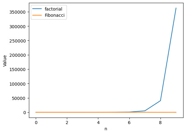
The factorial function grows much faster. In fact, you can’t even see the Fibonacci sequence. It’s not entirely surprising: a function where we multiply by n each iteration is bound to grow faster than one where we add (roughly) n each iteration.

Let’s plot these on a semilog plot so we can see them both a little more clearly:

You can do many more things with matplotlib. Check the docs for tutorials and examples.

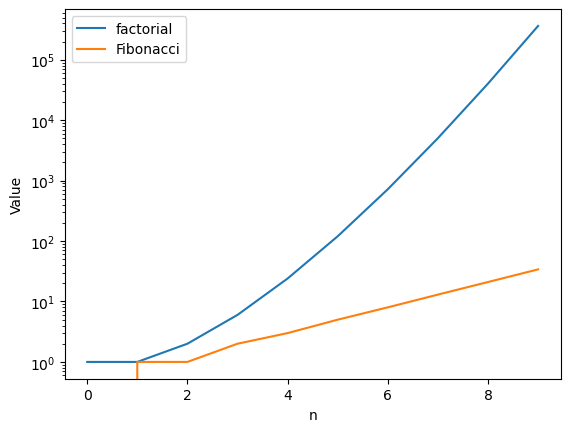
2Numpy and Scipy¶

Numpy contains core routines for doing fast vector, matrix, and linear algebra-type operations in Python. Scipy contains additional routines for optimization, special functions, and so on. Both contain modules written in C and Fortran to improve the performance.

First of all, we import numpy with

2.1Making vectors and matrices¶

Fundamental to both Numpy and Scipy is the ability to work with vectors, matrices or their generalisations, tensors. You can create arrays from lists using the np.array() function:

You can optionally pass in a second argument to np.array to choose a numeric type. There are a number of types listed here that your array can be, comprising integer (int, np.uint8 or np.int64, for instance) and floating point (e.g. float, np.float32 or np.complex64) types.

To build multidimensional arrays (such as matrices), you can use the array command with lists of lists:

You can also define arrays of arbitrary shape using the zeros command:

where the first argument is a tuple containing the shape of the array, and the second is the data type argument, which follows the same conventions as in the array command. Note that you can define either row or column vectors:

There’s also an identity command that behaves as you’d expect:

as well as a ones() function.

2.2Linspace, matrix functions, and plotting¶

The linspace command makes a linear array of a specified number of points from a starting to an ending value:

The optional third argument is the number of points, which defaults to 50.

linspace() is an easy way to make coordinates for plotting. Functions in the numpy library can act on an entire vector (or even a matrix) of points at once. Thus,

Note here that we used the numpy (and not the math) version of the sin function, which can take a vector of points. We also used the value of π built into the numpy library. This is a nice “recipe” to plot functions with matplotlib:

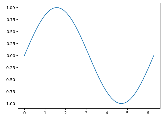
2.3Matrix operations¶

Matrix objects act sensibly when multiplied by scalars:

Same-shape matrices can be added together:

Note that the * operator acts in an element-wise way:

To get matrix multiplication, you use the @ operator:

There are determinant(), inverse(), and transpose() functions that act as you would suppose. Transpose can be abbreviated with .T at the end of a matrix object:

2.4Matrix Solvers¶

You can solve systems of linear equations using the np.linalg.solve() function:

There are also a number of routines to compute eigenvalues and eigenvectors that can be useful for scientific computing:

• eigvals() returns the eigenvalues of a matrix
• eigvalsh() returns the eigenvalues of a Hermitian matrix
• eig() returns the eigenvalues and eigenvectors of a matrix
• eigh() returns the eigenvalues and eigenvectors of a Hermitian matrix.

We know that the derivative of the sin function is the cos function. Let’s see whether this is the case using the numeric derivative:

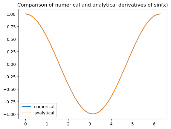
Pretty close!

2.5Monte Carlo, random numbers, and computing π¶

Many methods in scientific computing rely on Monte Carlo integration, where a sequence of (pseudo) random numbers are used to approximate the integral of a function. Python has good random number generators in the standard library. The random() function gives pseudorandom numbers uniformly distributed between 0 and 1:

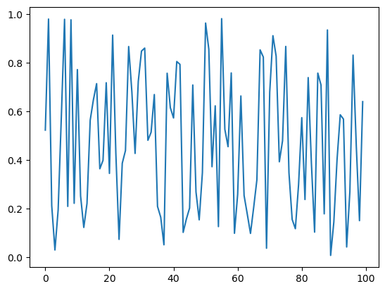
Note that random() uses the Mersenne Twister algorithm, which is more sophisticated (and has better statistical properties) than the linear congruential generator that C uses by default. There are also functions to generate random integers, to randomly shuffle a list, and functions to pick random numbers from a particular distribution, like the normal distribution:

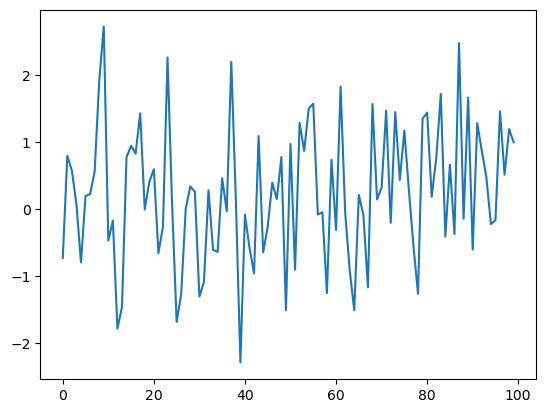
It is generally more efficient to generate a list of random numbers all at once, particularly if you’re drawing from a non-uniform distribution. Numpy has functions to generate vectors and matrices of particular types of random distributions.

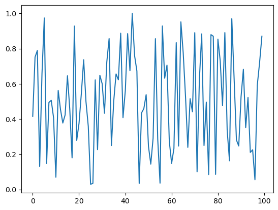
As an example, consider the following snippet, which estimates the value of π by taking random numbers as $x$ and $y$ coordinates, and counting how many of them are in the unit circle:

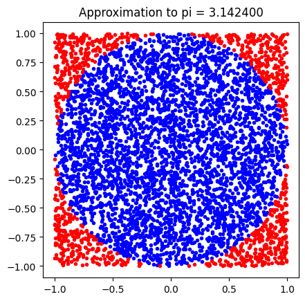
2.6Numerical Integration¶

Integration can be hard, and sometimes it’s easier to work out a definite integral using an approximation. For example, suppose we wanted to figure out the integral:

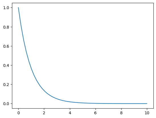
Scipy has a numerical integration routine quad() (since sometimes numerical integration is called quadrature) that we can use for this:

There are also 2d and 3d numerical integrators in Scipy. See the docs for more information.

3Intermediate Python¶

Consider the following (long) string:

First, note that the data is entered into a multi-line string. When Python sees three quote marks """ or ''' it treats everything following as part of a single string, including newlines, tabs, and anything else, until it sees the same three quote marks (""" has to be followed by another """, and ''' has to be followed by another ''') again.

We start by splitting this big string into a list of strings, since each line corresponds to a separate piece of data. We use split("\n"), which breaks a string into a new element every time it sees a newline (`\n) character:

We now want to do three things:

• Skip over the lines that don’t carry any information
• Break apart each line that does carry information and grab the pieces we want
• Turn the resulting data into something that we can plot.

For this data, we really only want the Energy column, the Gmax column (which contains the maximum gradient at each step), and perhaps the Walltime column.

Since the data is now in a list of lines, we can iterate over it:

Let’s examine what we just did: first, we used a for loop to iterate over each line. However, we skipped the first two, sincelines[2:] only takes the lines starting from index 2, since lines[0] contained the title information, and lines[1] contained underscores.

We then split each line into chunks (which we’re calling “words”, even though in most cases they’re numbers) using the string split() function on a string. If called without arguments, split() will split a string every time a whitespace is encountered:

This is almost exactly what we want. Now we can get the columns that we want:

This is fine for printing things out, but if we want to do something with the data, either make a calculation with it or pass it into a plotting, we need to convert the strings into regular floating point numbers. We can use the float() function for this. We also need to save it in some form. I’ll do this as follows:

We now have our data in a numpy array, so we can choose columns to print. With numpy matrices, multidimensional arrays can be accessed by using “slice tuples”. For instance, if we want the first column of a matrix such as data, we can use data[:,0]:

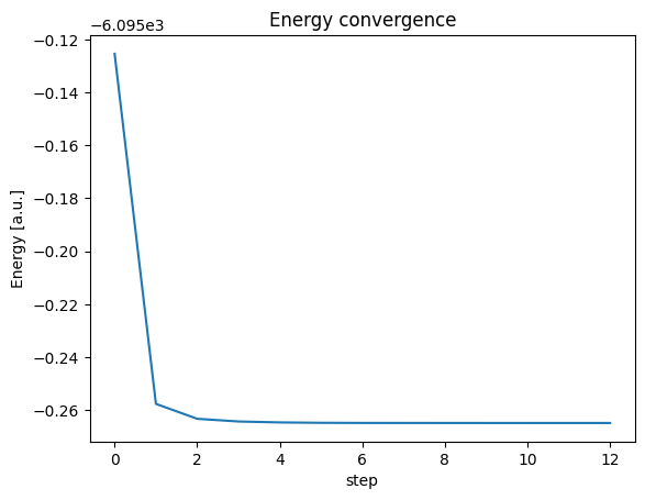
3.1More Sophisticated String Formatting and Processing¶

Strings are a big deal in most modern languages, and hopefully the previous sections helped underscore how versatile Python’s string processing techniques are. We will continue this topic in this chapter.

We can print out lines in Python using the print command.

In Jupyter notebooks we don’t even need the print command, since it will display the last expression not assigned to a variable.

print() even converts some arguments to strings for us:

As versatile as this is, you typically need more freedom over the data you print out. For example, what if we want to print a bunch of data to exactly 4 decimal places? We can do this using formatted strings.

Formatted strings share a syntax with the C printf statement. We make a string that has some funny format characters in it, and then pass a bunch of variables into the string that fill out those characters in different ways.

For example,

The other use of the percent sign is after the string, to pipe a set of variables in. You can pass in multiple variables (if your formatting string supports it) by putting a tuple after the percent. Thus,

3.2Optional arguments¶

You will recall that the linspace() function can take either two arguments (for the starting and ending points):

or it can take three arguments, for the starting point, the ending point, and the number of points:

You can also pass in keywords to exclude the endpoint:

Right now, we only know how to specify functions that have a fixed number of arguments. We’ll learn how to do the more general cases here.

If we’re defining a simple version of linspace, we would start with:

We can add an optional argument by specifying a default value in the argument list:

This gives exactly the same result if we don’t specify anything:

But also let’s us override the default value with a third argument:

We can add arbitrary keyword arguments to the function definition by putting a keyword argument **kwargs handle in:

What the keyword argument construction does is to take any additional keyword arguments (i.e. arguments specified by name, like endpoint=False), and stick them into a dictionary called kwargs (you can call it anything you like, but it has to be preceded by two stars). You can then grab items out of the dictionary using the get command, which also lets you specify a default value. I realize it takes a little getting used to, but it is a common construction in Python code, and you should be able to recognize it.

3.3List Comprehensions and Generators¶

List comprehensions are a streamlined way to make lists. They look something like a list definition, with some logic thrown in. For example:

You can also put some boolean testing into the construct:

These are useful building blocks for functional programming.

The lambda operator allows us to build anonymous functions, which are simply functions that aren’t defined by a normal def statement with a name. For example, a function that doubles the input is:

We could also write this as:

And assign it to a function separately:

lambda is particularly convenient (as we’ll see below) in passing simple functions as arguments to other functions.

map is a way to repeatedly apply a function to a list:

reduce is a way to repeatedly apply a function to the first two items of the list. There already is a sum function in Python that is a reduction:

We can use reduce to define an analogous prod function:

3.4Object Oriented Programming¶

We’ve seen a lot of examples of objects in Python. We create a string object with quote marks:

and we have a bunch of methods we can use on the object:

Object oriented programming simply gives you the tools to define objects and methods for yourself. It’s useful anytime you want to keep some data (like the characters in the string) tightly coupled to the functions that act on the data (length, split, startswith, etc.).

As an example, we can write a very primitive immutable 3D vector:

The __init__() function specifies the operations to perform when the object is created. The self argument is the object itself, and we don’t pass it in. Note that we define some functions to access the three coordinates, as well as a function to compute the dot product. Finally, we “overload” two operators, + and -. The class can be used like this: